Multiclass Object Detection Using YOLO v2 Deep Learning
This example shows how to perform multiclass object detection on a custom data set and evaluate performance metrics.
Overview
Deep learning is a powerful machine learning technique that you can use to train robust multiclass object detectors such as YOLO v2, YOLO v4, YOLOX, RTMDet, and SSD. This example trains a YOLO v2 multiclass object detector using the trainYOLOv2ObjectDetector function. The trained object detector is able to detect and identify multiple indoor objects. For more information about training other multiclass object detectors, such as YOLOX, YOLO v4, SSD, and Faster R-CNN, see Get Started with Object Detection Using Deep Learning and Choose an Object Detector.
This example first shows you how to detect multiple objects in an image using a pretrained YOLO v2 object detector. Then, you can optionally download a data set and train YOLO v2 on a custom data set using transfer learning.
Load Pretrained Object Detector
Download a pretrained YOLO v2 object detector, and load it into the workspace.
pretrainedURL = "https://www.mathworks.com/supportfiles/vision/data/yolov2IndoorObjectDetector23b.zip";
pretrainedFolder = fullfile(tempdir,"pretrainedNetwork");
pretrainedNetworkZip = fullfile(pretrainedFolder,"yolov2IndoorObjectDetector23b.zip");

if ~exist(pretrainedNetworkZip,"file")
    mkdir(pretrainedFolder)
    disp("Downloading pretrained network (6 MB)...")
    websave(pretrainedNetworkZip,pretrainedURL)
end

unzip(pretrainedNetworkZip,pretrainedFolder)

trainedNetwork = fullfile(pretrainedFolder,"yolov2IndoorObjectDetector.mat");
trainedNetwork = load(trainedNetwork);
trainedDetector = trainedNetwork.detector;
Detect Multiple Indoor Objects
Read a test image that contains objects of the target classes, run the object detector on the image, and display an image annotated with the detection results.
I = imread("indoorTest.jpg");
[bbox,score,label] = detect(trainedDetector,I);

LabelScoreStr = compose("%s-%.2f",label,score);
annotatedImage = insertObjectAnnotation(I,"rectangle",bbox,LabelScoreStr,LineWidth=4,FontSize=24);
figure
imshow(annotatedImage)

Load Data for Training
This example uses the Indoor Object Detection Dataset created by Bishwo Adhikari [1]. The data set consists of 2213 labeled images collected from indoor scenes and contains 7 classes: fire extinguisher, chair, clock, trash bin, screen, and printer. Each image contains one or more labeled instances of these classes. Check whether the data set has already been downloaded and, if it is not, use websave to download it.
dsURL = "https://zenodo.org/record/2654485/files/Indoor%20Object%20Detection%20Dataset.zip?download=1";
outputFolder = fullfile(tempdir,"indoorObjectDetection");
imagesZip = fullfile(outputFolder,"indoor.zip");

if ~exist(imagesZip,"file")
    mkdir(outputFolder)
    disp("Downloading 401 MB Indoor Objects Dataset images...")
    websave(imagesZip,dsURL)
    unzip(imagesZip,fullfile(outputFolder))
end
Create an imageDatastore object to store the images from the data set.
datapath = fullfile(outputFolder,"Indoor Object Detection Dataset");
imds = imageDatastore(datapath,IncludeSubfolders=true, FileExtensions=".jpg");
The annotationsIndoor.mat file contains annotations for each of the images in the data, as well as vectors that specify the indices of the data set images to use for the training, validation, and test sets. Load the file into the workspace, and extract annotations and the indices corresponding to the training, validation, and test sets from the data variable. The indices specify 2207 images in total, instead of 2213 images, as 6 images have no labels associated with them. Use the indices of the images that contain labels to remove these 6 images from the image and annotations datastores.
data = load("annotationsIndoor.mat");
blds = data.BBstore;
trainingIdx = data.trainingIdx;
validationIdx = data.validationIdx;
testIdx = data.testIdx;
cleanIdx = data.idxs;

% Remove the 6 images with no labels.
imds = subset(imds,cleanIdx);
blds = subset(blds,cleanIdx);
Analyze Training Data
Analyze the distribution of object class labels and sizes to understand the data better. This analysis is critical because it helps you determine how to prepare the training data and how to configure an object detector for this specific data set.
Analyze Class Distribution
Measure the distribution of bounding box class labels in the data set by using the countEachLabel function.
tbl = countEachLabel(blds)
tbl=7×3 table
                exit     545    504
    fireextinguisher    1684    818
               chair    1662    850
               clock     280    277
            trashbin     228    170
              screen     115     94
             printer      81     81
Visualize the counts by class.
bar(tbl.Label,tbl.Count)
ylabel("Frequency")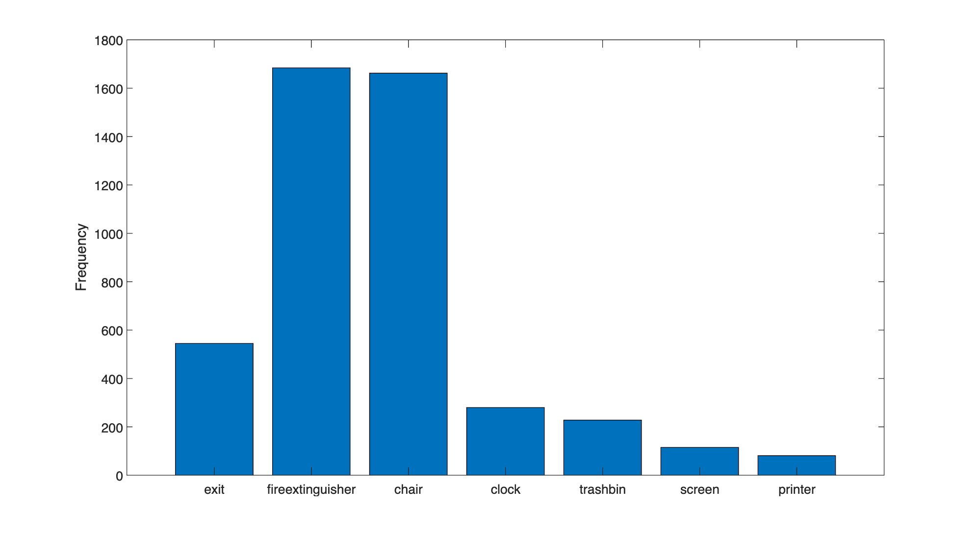
The classes in this data set are unbalanced. This imbalance can be detrimental to the learning process because the process is biased in favor of the dominant classes. To address the imbalance, use one or more of these complementary techniques: add more data, oversample the underrepresented classes, modify the loss function, or apply data augmentation. Regardless of which approach you use, you must perform empirical analysis to determine the optimal solution for your data set. In this example, you will use data augmentation to reduce bias in the learning process.
Analyze Object Sizes and Choose Object Detector
Read all the bounding boxes and labels within the data set, and calculate the diagonal length of the bounding box.
data = readall(blds);
bboxes = vertcat(data{:,1});
labels = vertcat(data{:,2});
diagonalLength = hypot(bboxes(:,3),bboxes(:,4));
Group the object lengths by class.
G = findgroups(labels);
groupedDiagonalLength = splitapply(@(x){x},diagonalLength,G);
Visualize the distribution of object lengths for each class.
figure
classes = tbl.Label;
numClasses = numel(classes);
for i = 1:numClasses
    len = groupedDiagonalLength{i};
    x = repelem(i,numel(len),1);
    plot(x,len,"o")
    hold on
end
hold off
ylabel("Object extent (pixels)")

xticks(1:numClasses)
xticklabels(classes)
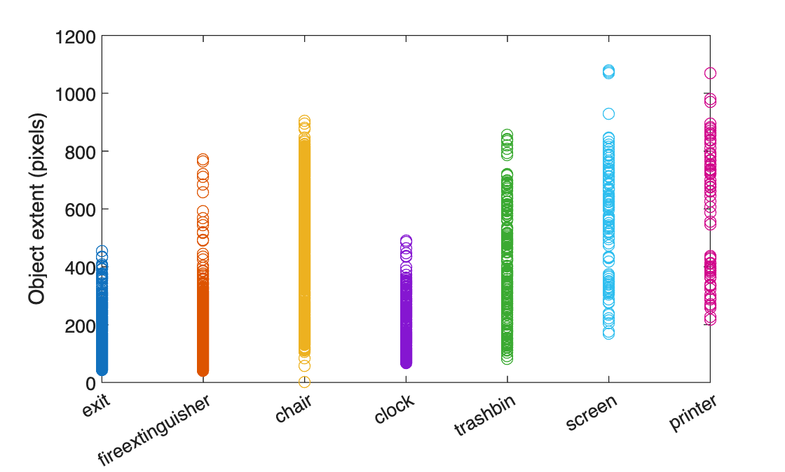
This visualization highlights the important data set attributes that help you determine which type of object detector to configure:
The object size variance within each class
The object size variance across classes
This data set has a good amount of overlap between the size ranges across classes. In addition, the size variation within each class is not very large. This means that you can train one multiclass detector to handle a range of object sizes. If the size ranges do not overlap, or if the range of object sizes differs by an order of magnitude, then it is more practical to train multiple detectors for different size ranges.
You can determine which object detector to train based on the size variance. When size variance within each class is small, use a single-scale object detector such as YOLO v2. If each class contains large variance, choose a multi-scale object detector such as YOLO v4 or SSD. Since the object sizes in this data set are within the same order of magnitude, use YOLO v2 to start. Although advanced multi-scale detectors might perform better, training them can take more time and resources than YOLO v2. Use more advanced detectors when simpler solutions do not meet your performance requirements.
Use the size distribution information to select the training image size. A fixed size enables batch processing during training. The training image size dictates how large the batch size can be based on the resource constraints of your training environment, such as GPU memory. Process larger batches of data to improve throughput and reduce training time, especially when using a GPU. However, the training image size can impact the resolution of objects if you drastically resize the original data to a smaller size.
In the following section, configure a YOLO v2 object detector using the size analysis information for this data set.
Define YOLO v2 Object Detector Architecture
Configure a YOLO v2 object detector using these steps:
Choose a pretrained detector for transfer learning.
Choose a training image size.
Select which network features to use for predicting object locations and classes.
Estimate anchor boxes from the preprocessed data used to train the object detector.
Select a pretrained Tiny YOLO v2 detector for transfer learning. Tiny YOLO v2 is a lightweight network trained on COCO [2], a large object detection data set. Transfer learning using a pretrained object detector reduces training time compared to training a network from scratch. Alternatively, you can use the larger Darknet-19 YOLO v2 pretrained detector, but consider starting with a simpler network to establish a performance baseline before experimenting with a larger network. Using the Tiny or Darknet-19 YOLO v2 pretrained detector requires the Computer Vision Toolbox™ Model for YOLO v2 Object Detection.
pretrainedDetector = yolov2ObjectDetector("tiny-yolov2-coco");Next, choose the size of the training images for YOLO v2. When choosing the training image size, consider these size parameters:
The distribution of object sizes in the images, and the impact of resizing the images on the object sizes.
The computational resources required to batch process data at the selected size.
The minimum input size required by the network.
Determine the input size of the pretrained Tiny YOLO v2 network.
pretrainedDetector.Network.Layers(1).InputSize
ans = 1×3

    416    416    3
The size of the images within the Indoor Object Detection Dataset is [720 1024 3]. Based on your object analysis, the smallest objects are approximately 20-by-20 pixels.
To maintain a balance between accuracy and the computational cost of running the example, specify a size of [720 720 3]. This size ensures that resizing each image does not drastically affect the spatial resolution of objects in this data set. If you adapt this example for your own data set, you must change the training image size based on your data. Determining the optimal input size requires empirical analysis.
inputSize = [720 720 3];
Combine the image and bounding box datastores.
ds = combine(imds,blds);
Use transform to apply a preprocessing function that resizes images and their corresponding bounding boxes. The function also sanitizes the bounding boxes to convert them to a valid shape.
preprocessedData = transform(ds,@(data)resizeImageAndLabel(data,inputSize));
Display one of the preprocessed images and its bounding box labels to verify that the objects in the resized images still have visible features.
data = preview(preprocessedData);
I = data{1};
bbox = data{2};
label = data{3};
imshow(I)
showShape("rectangle",bbox,Label=label)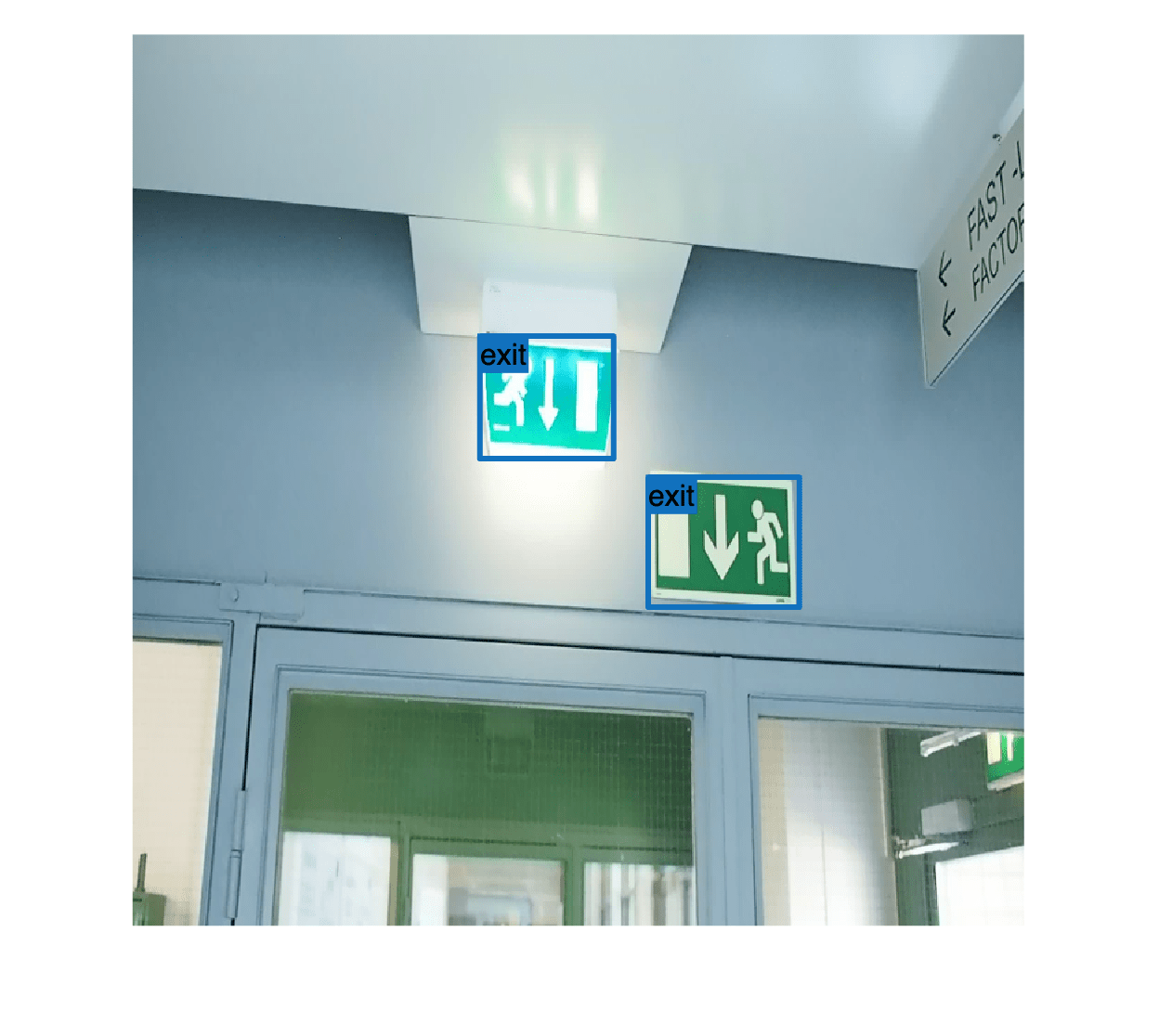
YOLO v2 is a single-scale detector because it uses features extracted from one network layer to predict the location and class of objects in the image. The feature extraction layer is an important hyperparameter for deep learning based object detectors. When selecting the feature extraction layer, choose a layer that outputs features at a spatial resolution that is suitable for the range of object sizes in the data set.
Most networks used in object detection spatially downsample features by powers of two as the data flows through the network. For example, starting from the specified input size, networks can have layers that produce feature maps downsampled spatially by 4x, 8x, 16x, and 32x. If object sizes in the data set are small (for example, less than 10-by-10 pixels), feature maps downsampled by 16x and 32x might not have sufficient spatial resolution to locate the objects precisely. Conversely, if the objects are large, feature maps downsampled by 4x or 8x might not encode enough global context for those objects.
For this data set, specify the "leaky_relu_5" layer of the Tiny YOLO v2 network, which outputs feature maps downsampled by 16x. This amount of downsampling is a good trade-off between spatial resolution and the strength of the extracted features, as features extracted further down the network encode stronger image features at the cost of spatial resolution.
featureLayer = "leaky_relu_5";You can use the analyzeNetwork (Deep Learning Toolbox) function to visualize the Tiny YOLO v2 network and determine the name of the layer that outputs features downsampled by 16x.
Next, use estimateAnchorBoxes to estimate anchor boxes from the training data. Estimating anchor boxes from the preprocessed data enables you to get an estimate based on the selected training image size. You can use the procedure defined in the Estimate Anchor Boxes from Training Data example to determine the number of anchor boxes suitable for the data set. Based on this procedure, five anchor boxes is a good trade-off between computational cost and accuracy. As with any other hyperparameter, you must optimize the number of anchor boxes for your data using empirical analysis.
numAnchors = 5;
aboxes = estimateAnchorBoxes(preprocessedData,numAnchors);
Finally, configure the YOLO v2 network for transfer learning on seven classes with the selected training image size, and estimated anchor boxes.
pretrainedNet = pretrainedDetector.Network;
classes = {'exit','fireextinguisher','chair','clock','trashbin','screen','printer'};
detector = yolov2ObjectDetector(pretrainedNet,classes,aboxes, ...
DetectionNetworkSource=featureLayer,InputSize= inputSize);You can visualize the network using the analyzeNetwork (Deep Learning Toolbox) function or Deep Network Designer (Deep Learning Toolbox) app.
Prepare Training Data
Initialize the random number generator with a seed of 0 using rng, and shuffle the data set for reproducibility using the shuffle function.
rng(0);
preprocessedData = shuffle(preprocessedData);
Split the data set into training, test, and validation subsets using the subset function.
dsTrain = subset(preprocessedData,trainingIdx);
dsVal = subset(preprocessedData,validationIdx);
dsTest = subset(preprocessedData,testIdx);
Data Augmentation
Use data augmentation to improve network accuracy by randomly transforming the original data during training. Data augmentation enables you to add more variety to the training data without increasing the number of labeled training samples. Use transform to augment the training data using these steps:
Randomly flip the image and associated bounding box labels horizontally.
Randomly scale the image and associated bounding box labels.
Jitter the image color.
augmentedTrainingData = transform(dsTrain,@augmentData);
Display one of the training images and box labels.
data = read(augmentedTrainingData);
I = data{1};
bbox = data{2};
label = data{3};
imshow(I)
showShape("rectangle",bbox,Label=label)
Train YOLOv2 Object Detector
Specify the network training options using the trainingOptions (Deep Learning Toolbox) function.
opts = trainingOptions("rmsprop", ...
        InitialLearnRate=0.001, ...
        MiniBatchSize=8, ...
        MaxEpochs=10, ...
        LearnRateSchedule="piecewise", ...
        LearnRateDropPeriod=5, ...
        VerboseFrequency=30, ...
        L2Regularization=0.001, ...
        ValidationData=dsVal, ...
        ValidationFrequency=50, ...
        OutputNetwork="best-validation-loss");
These training options have been selected using Experiment Manager. For more information on using Experiment Manager for hyperparameter tuning, see Train Object Detectors in Experiment Manager.
To use the trainYOLOv2ObjectDetector function to train a YOLO v2 object detector, set doTraining is set to true.
doTraining = false;
if doTraining
    [detector,info] = trainYOLOv2ObjectDetector(augmentedTrainingData,detector,opts);
else
    detector = trainedDetector;
end
This example was verified on an NVIDIA™ GeForce RTX 3090 Ti GPU with 24 GB of memory, which required approximately 45 minutes to complete training. Training time varies depending on the hardware you use. If your GPU has less memory, you may run out of memory. To use less memory, specify a lower MiniBatchSize value when using the trainingOptions (Deep Learning Toolbox) function.
Evaluate Object Detector
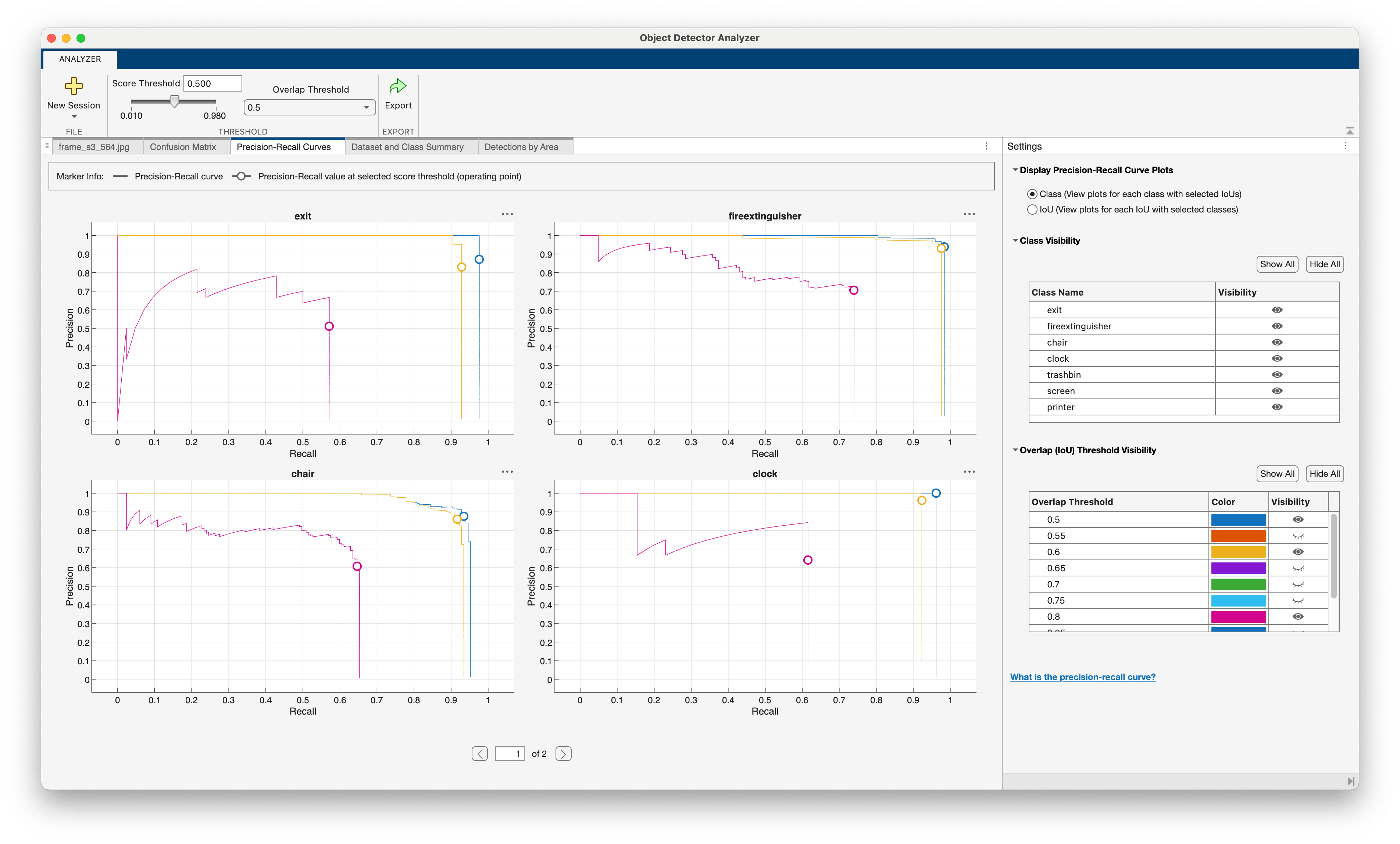
Use the Object Detector Analyzer app to visualize and evaluate the performance of the detector against ground truth. The app runs the detector on the test set and computes metrics such as AP and mAP, plots precision-recall curves, and displays the detections on each image in the test set. You can visualize ground truth data alongside correct and incorrect detector predictions and quickly navigate to images where the detector made the most mistakes to better understand the performance. For example, the detector may fail in specific scenarios that may indicate that the detector should be retrained with additional data that includes those specific scenarios. To learn more about performance metrics, see Evaluate Object Detector Performance.
To launch the app, use the objectDetectorAnalyzer function.
objectDetectorAnalyzer(detector,dsTest)
Select the Precision-Recall Curves tab to see the precision-recall (PR) curves for each class. The curves show that the detector performs well on the test set when the overlap threshold for evaluation is 0.5, but performance degrades as the overlap threshold increases to 0.7 and 0.8. The circular markers on each curve indicate the operating point of the detector. An operating point on a PR curve is a specific detection score threshold setting that determines the balance between precision and recall achieved by the detector. You can adjust the score threshold slider to determine the optimal operating point for your application.
Explore the other tabs to see additional detection metrics:
Dataset and Class Summary: Summarizes the performance of the dataset across all classes.
Confusion Matrix: Displays the number of objects found and missed for each class.
Detections by Area: Visualize correct and incorrect detections per object size area range to spot detection error trends due to object size.
Evaluate Object Size Impact on Detector Performance
Click the Export button to export the detection metrics to the workspace as an objectDetectionMetrics object, metrics. Investigate the impact of object size on detector performance by using the exported metrics and the metricsByArea object function, which computes performance metrics for specific object size ranges. You can specify the object size range based on a predefined set of size ranges for your application, or use the estimated anchor boxes as in this example. The anchor box estimation method automatically clusters the object sizes and provides a set of size ranges based on the input data.
Load pre-computed metrics if they are not found in the workspace.
if ~exist("metrics","var")
    loadedMetrics = load("metricsIndoorObjectsYOLOv2.mat")
    metrics = loadedMetrics.metrics;
end
Extract the anchor boxes from the detector, calculate their areas, and sort the areas.
areas = prod(detector.AnchorBoxes,2);
areas = sort(areas);
Define area range limits using the calculated areas. The upper limit for the last range is set to three times the size of the largest area, which is sufficient for the objects in this data set.
lowerLimit = [0; areas];
upperLimit = [areas; 3*areas(end)];
areaRanges = [lowerLimit upperLimit]
areaRanges = 6×2

         0      2774
      2774      9177
      9177     15916
     15916     47799
     47799    124716
    124716    374148
Evaluate the object detection metrics across the defined size ranges for the chair class by using the metricsByArea function. You can specify other class names to evaluate the object detection metrics for those classes interactively using the drop-down value selector for the ClassName name-value argument.
classes = string(detector.ClassNames);
areaMetrics = metricsByArea(metrics,areaRanges,ClassName= classes(1))
areaMetrics=6×6 table
         0      2774    15    0.5493                   [1;1;0.8578;0.7684;0.7684;0.4540;0.3913;0.2533;0;0]                               10×2321 double                               10×2321 double
      2774      9177    18    0.6048    [0.9444;0.9444;0.9444;0.9444;0.9444;0.6861;0.4733;0.1263;0.0401;0]                                10×651 double                                10×651 double
      9177     15916     5    0.6300                             [1;1;1;1;1;0.7600;0.1800;0.1800;0.1800;0]                                10×123 double                                10×123 double
     15916     47799     4    0.7375                                            [1;1;1;1;1;1;1;0.3750;0;0]                                10×159 double                                10×159 double
     47799    124716     0         0                                                 [0;0;0;0;0;0;0;0;0;0]                                 10×30 double                                 10×30 double
    124716    374148     0       NaN                             [NaN;NaN;NaN;NaN;NaN;NaN;NaN;NaN;NaN;NaN]    [NaN;NaN;NaN;NaN;NaN;NaN;NaN;NaN;NaN;NaN]    [NaN;NaN;NaN;NaN;NaN;NaN;NaN;NaN;NaN;NaN]
The NumObjects column shows how many objects in the test data set fall within the area range. Although the detector performed well on the chair class overall, there is a size range where the detector has low average precision compared to the other size ranges. The range where the detector does not perform well has only 11 samples. To improve the performance in this size range, add more samples of this size to the training data, or use data augmentation to create more samples across the set of size ranges.
For more insight into how to improve detector performance, you can examine the size-based metrics for other classes.
Deployment
Once the detector has been trained and evaluated, you can optionally generate code and deploy the yolov2ObjectDetector using GPU Coder™. For more information, see Code Generation for Object Detection by Using YOLO v2 (GPU Coder) example.
Summary
This example shows how to train and evaluate a multiclass object detector. When adapting this example to your own data, carefully assess the object class and size distribution in your data set. Your data might require using different hyperparameters or a different object detector, such as YOLO v4 or YOLOX, for optimal results.
Supporting Functions
function B = augmentData(A)
% Apply random horizontal flipping, and random X/Y scaling, and jitter image color.
% The function clips boxes scaled outside the bounds if the overlap is above 0.25.
B = cell(size(A));

I = A{1};
sz = size(I);
if numel(sz)==3 && sz(3) == 3
    I = jitterColorHSV(I, ...
        Contrast=0.2, ...
        Hue=0, ...
        Saturation=0.1, ...
        Brightness=0.2);
end

% Randomly flip and scale image.
tform = randomAffine2d(XReflection=true,Scale=[1 1.1]);
rout = affineOutputView(sz,tform,BoundsStyle="CenterOutput");
B{1} = imwarp(I,tform,OutputView=rout);

% Sanitize boxes, if needed. This helper function is attached to the example as a
% supporting file. Open the example in MATLAB to use this function.
A{2} = helperSanitizeBoxes(A{2});

% Apply same transform to boxes.
[B{2},indices] = bboxwarp(A{2},tform,rout,OverlapThreshold=0.25);
B{3} = A{3}(indices);

% Return original data only when all boxes have been removed by warping.
if isempty(indices)
    B = A;
end
end
function data = resizeImageAndLabel(data,targetSize)
% Resize the images, and scale the corresponding bounding boxes.

    scale = (targetSize(1:2))./size(data{1},[1 2]);
    data{1} = imresize(data{1},targetSize(1:2));
    data{2} = bboxresize(data{2},scale);

    data{2} = floor(data{2});
    imageSize = targetSize(1:2);
    boxes = data{2};
    % Set boxes with negative values to have value 1.
    boxes(boxes <= 0) = 1;

    % Validate if bounding box in within image boundary.
    boxes(:,3) = min(boxes(:,3),imageSize(2) - boxes(:,1) - 1);
    boxes(:,4) = min(boxes(:,4),imageSize(1) - boxes(:,2) - 1);

    data{2} = boxes;

end
References
[1] Adhikari, Bishwo; Peltomaki, Jukka; Huttunen, Heikki. (2019). Indoor Object Detection Dataset [Data set]. 7th European Workshop on Visual Information Processing 2018 (EUVIP), Tampere, Finland.
[2] Lin, Tsung-Yi, Michael Maire, Serge Belongie, Lubomir Bourdev, Ross Girshick, James Hays, Pietro Perona, Deva Ramanan, C. Lawrence Zitnick, and Piotr Dollár. “Microsoft COCO: Common Objects in Context,” May 1, 2014. https://arxiv.org/abs/1405.0312v3.
See Also
Apps
Functions
evaluateObjectDetection|objectDetectionMetrics|averagePrecision|confusionMatrix|metricsByArea
See Also
Topics
- Evaluate Object Detector Performance
- Get Started with Object Detector Analyzer
- Object Detection in Large Satellite Imagery Using Deep Learning
- Object Detection Using YOLO v4 Deep Learning
- Detect Defects on Printed Circuit Boards Using YOLOX Network
- Choose an Object Detector
- Get Started with Object Detection Using Deep Learning