Dense 3-D Reconstruction from Multiple Views Using RAFT Optical Flow
This example demonstrates multi-view dense 3-D reconstruction [1] by combining structure-from-motion (SfM) results with dense pixel-wise correspondences from RAFT optical flow [2].
The example follows these steps:
Select optimal view pairs for dense depth estimation by traversing the view graph obtained from SfM.
Compute optical flow on the selected view pairs.
Enforce geometric consistency checks on optical flow estimates.
Estimate dense depth by triangulation using relative camera pose and optical flow between view pairs.
Reject regions of uncertain depth estimation.
Fuse all individual depth estimates and corresponding RGB values into a single colored point cloud.
This process results in a fast and accurate pipeline for dense reconstruction, leveraging the compute capabilities of a GPU when available. Techniques such as Neural Radiance Field (NeRF) provide denser point clouds, often at better quality, at the cost of significantly longer processing times and hardware requirements such as a GPU with at least 16 GB memory. For more information on using NeRF for 3-D reconstruction, see Reconstruct 3-D Scenes and Synthesize Novel Views Using Neural Radiance Field Model.
Download and Unzip Training Data
This example uses a subset of the TUM RGB-D Benchmark [3] containing 104 images of an indoor office scene captured with a handheld camera. You can download the data to a temporary directory using a web browser or by running this code:
if ~exist("tum_rgbd_data.zip", "file")
    websave("tum_rgbd_data.zip", "https://ssd.mathworks.com/supportfiles/3DReconstruction/tum_rgbd_data.zip");
    unzip(fullfile("tum_rgbd_data.zip"), pwd);
end

if ~exist(fullfile("sfmTrainingDataTUMRGBD", "finalReconstructionSfM.mat"), "file")
    websave(fullfile("sfmTrainingDataTUMRGBD", "finalReconstructionSfM.mat"),...
        "https://ssd.mathworks.com/supportfiles/supportfiles/3DReconstruction/finalReconstructionSfM.mat");
end
Load Data and Structure-from-Motion Results
This example builds on the view graph and sparse point clouds created in the Structure from Motion from Multiple Views example. Ensure that the images used in the SfM example are available on the path.
Load the camera intrinsics, image view graph, and reconstructed sparse world points from the saved SfM results.
load(fullfile("sfmTrainingDataTUMRGBD", "cameraInfo.mat"), "intrinsics");
load(fullfile("sfmTrainingDataTUMRGBD", "finalReconstructionSfM.mat"), "viewGraph", "wpSet");
Create an image datastore to load the images of the scene.
imds = imageDatastore(fullfile("sfmTrainingDataTUMRGBD","images"));
numImages = length(imds.Files);
numConn = viewGraph.NumConnections;
numViews = viewGraph.NumViews;
Create opticalFlowRAFT Object
Create an opticalFlowRAFT model for computing dense pixel correspondences between image pairs.
raft = opticalFlowRAFT;
Select View Pairs for Dense Depth Estimation Using the SfM View Graph
For each image in the image collection, select its neighboring view most suitable for dense reconstruction. Dense reconstruction depends on finding pixel-wise matches between two images and then triangulating to obtain 3-D points in world coordinates for each of the matched pixels. A numerically stable triangulation computation requires the two views to have sufficient viewpoint variation between the two camera positions, along with a minimum number of mutually visible image features.
The minOverlap threshold rejects view pairs that are too far apart and do not share common features. The ideal value is data set dependent and has to be tuned to obtain a reasonable number of pairs covering multiple viewpoints for subsequent dense reconstruction. Reduce this threshold to consider more image pairs as valid for dense depth estimation. For more control over the view selection process, tune the parameters present in the helperSelectDepthViewPairs helper function, attached to this example as a supporting file
minOverlap = 0.2;
validViewPairs = helperSelectDepthViewPairs(viewGraph, wpSet, minOverlap);

numValidViewPairs = size(validViewPairs,1);
disp(numValidViewPairs + " valid views out of " + numViews+".");
78 valid views out of 104.
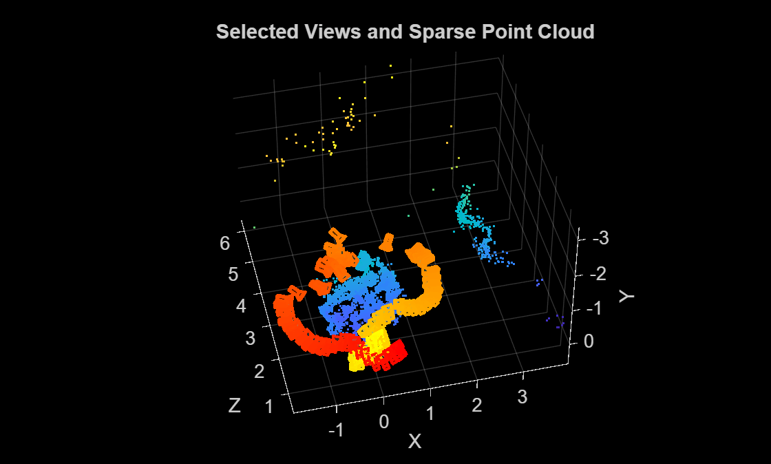
Visualize Selected View Pairs and Sparse Reconstruction
Visualize the selected views, along with the sparse 3-D points from SfM, to ensure that the object of interest has been captured from multiple viewpoints.
figure
pcshow(wpSet.WorldPoints, VerticalAxis="y", VerticalAxisDir="down");
xlabel("X")
ylabel("Y")
zlabel("Z")
hold on
camColors = autumn(numValidViewPairs);
for i = 1:numValidViewPairs
    viewId = validViewPairs(i,1);
    plotCamera(AbsolutePose=viewGraph.Views.AbsolutePose(viewId), Size=0.1, Color=camColors(i,:));
end
hold off
title("Selected Views and Sparse Point Cloud")
Estimate Depth Map from Image Pair
To compute a dense depth map between two views in the multi-view reconstruction sequence, first extract the camera poses and keypoint correspondences obtained from the earlier Structure-from-Motion (SfM) stage. The relative pose between the selected image pair defines the geometric relationship needed to triangulate dense pixel correspondences estimated using optical flow from the RAFT model. Because depths derived from optical-flow are determined only up to an unknown scale, you must then align and scale the resulting depth map to match the sparse 3-D points reconstructed by SfM. Finally, apply spatial filtering and superpixel-based region rejection to reduce noise, remove low-texture regions, and preserve depth boundaries.
Use the slider to select a particular image pair and compute a depth map of the first image using dense optical flow and triangulation from the relative camera pose between the two images.
pairIndex =29; viewPair = validViewPairs(pairIndex,:); % Thresholds tuned according to dataset maxDepthThreshold = 2; % reject depth at points that are too far away to be estimated correctly medianFilterSize = [5 5]; % size of the median filter kernel used to smooth the raw depth map numSuperPixels = 50; % number of super-pixels computed in an image to reject regions of low texture % Extract 3D World Points seen in view1 from the SfM results [pointIndices, featureIndices] = findWorldPointsInView(wpSet, viewPair(1)); xyzPoints = wpSet.WorldPoints(pointIndices,:); % Extract 2D keypoints detected in view1 from the SfM results view1 = findView(viewGraph, viewPair(1)); view2 = findView(viewGraph, viewPair(2)); featurePoints = view1.Points{:}(featureIndices); I1 = readimage(imds, viewPair(1)); I2 = readimage(imds, viewPair(2)); % Compute relative pose between camera positions of the two views pose1 = view1.AbsolutePose; pose2 = view2.AbsolutePose; p1Inv = invert(pose1); relPose = p1Inv.A * pose2.A; relPose = rigidtform3d(relPose); % Compute depth map using dense pixel correspondences from optical flow and % relative camera pose between two views. [depthMap, flow, isValid] = helperComputeDepthMap(... raft, I1, I2, relPose, intrinsics, featurePoints, maxDepthThreshold); % Scale the estimated depth map values to the same coordinates as the % sparse SfM keypoints. scaleFactor = helperComputeDepthMapScale(featurePoints, pose1, xyzPoints, depthMap); depthMap = scaleFactor * depthMap; % Median filtering to remove noise in local neighborhoods depthMap = medfilt2(depthMap, medianFilterSize); % SLIC superpixels to reject regions that have low texture and likely to % have incorrect estimates of depth. if numSuperPixels > 0 [L,N] = superpixels(I1, numSuperPixels); BW = boundarymask(L); depthMap = helperFilterSuperpixels(L, depthMap, featurePoints.Location); end
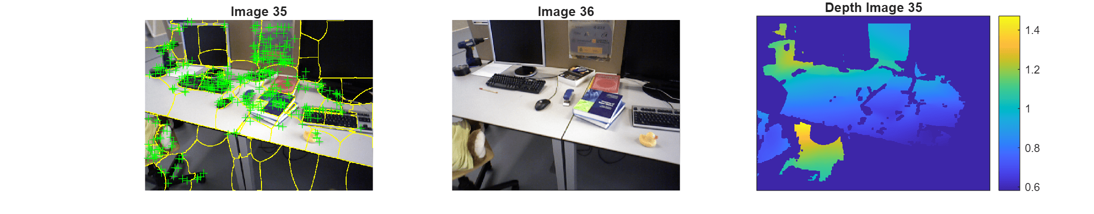
Visualize the two images and the estimated depth map. Invalid depth map pixels are marked using NaN values. The default thresholds in this example are set to very conservative values that reject a large number of regions in an image where depth estimates may be uncertain. This is done to avoid a noisy point cloud in the final result. In less challenging scenarios, these thresholds can be relaxed and stages such as the superpixel rejection may be omitted altogether without impacting the final reconstruction.
figure
subplot(1,3,1)
imshow(imoverlay(I1,BW,"yellow"))
hold on
plot(featurePoints,ShowScale=false)
hold off
title("Image " + viewPair(1))
subplot(1,3,2)
imshow(I2)
title("Image " + viewPair(2))
subplot(1,3,3)
imagesc(depthMap)
axis image
colorbar
xticks([])
yticks([])
title("Depth Image " + viewPair(1))
truesize;
Dense Reconstruction on Entire Image Sequence
Run the reconstruction algorithm on all the valid image pairs in the image sequence and reconstruct a dense point cloud. Two-view reconstructions from all the selected views, along with their color or intensity information, are concatenated into a single point cloud.
Executing this section of the code takes about 7 minutes on a Linux® machine with an NVIDIA® GeForce RTX 3090 GPU.
% Specify parameters
offset = 50;                         % Ignore image points at the boundary
depthRange = [0 maxDepthThreshold];  % Determined by visually inspecting the earlier individual depth maps

ptCloudsFull = cell(numValidViewPairs,1);
imageSize = size(I1);
[X, Y] = meshgrid(offset:2:imageSize(2)-offset, offset:2:imageSize(1)-offset);

for i = 1:numValidViewPairs

    viewPair = validViewPairs(i,:);

    fprintf(i + "/" + numValidViewPairs + " ");
    if mod(i,20) == 0
        fprintf("\n");
    end

    I1 = readimage(imds, viewPair(1));
    I2 = readimage(imds, viewPair(2));

    view1 = findView(viewGraph, viewPair(1));
    view2 = findView(viewGraph, viewPair(2));

    % 3D world points visible from view1
    [pointIndices, featureIndices] = findWorldPointsInView(wpSet, viewPair(1));
    xyzPoints = wpSet.WorldPoints(pointIndices,:);

    % 2D keypoints for visible world points in view1
    featurePoints = view1.Points{:}(featureIndices);

    % Camera poses of the two views
    pose1 = view1.AbsolutePose;
    pose2 = view2.AbsolutePose;

    % Compute relative pose between cameras
    p1Inv = invert(pose1);
    relPose = p1Inv.A * pose2.A;
    relPose = rigidtform3d(relPose);

    % Compute depth map using dense pixel correspondences from optical flow
    % and relative camera pose between two views from SfM.
    [depthMap, flow, isValid] = helperComputeDepthMap(...
        raft, I1, I2, relPose, intrinsics, featurePoints, depthRange(2));

    if ~isValid
        % Numerically unstable depth estimation
        continue;
    end

    % Scale the estimated depth map values to the same coordinates as the
    % sparse SfM keypoints.
    scaleFactor = helperComputeDepthMapScale(featurePoints,pose1,xyzPoints,depthMap);
    depthMap = scaleFactor * depthMap;

    % Median filtering to remove noise in local neighborhoods
    depthMap = medfilt2(depthMap, medianFilterSize);

    % SLIC superpixels to reject regions that have low texture and likely to
    % have incorrect estimates of depth.
    if numSuperPixels > 0
            [L,N] = superpixels(I1, numSuperPixels);
            BW = boundarymask(L);
            depthMap = helperFilterSuperpixels(L, depthMap, featurePoints.Location);
    end

    % Create a colored point cloud from the depth map of a single view
    [xyzPoints, validIndex] = helperReconstructFromRGBD([X(:), Y(:)], ...
        depthMap, intrinsics, pose1, 1, depthRange);
    colors = zeros(numel(X), 1, 'like', I1);
    for j = 1:numel(X)
        colors(j, 1:3) = I1(Y(j), X(j), :);
    end
    ptCloudOneView = pointCloud(xyzPoints, Color=colors(validIndex, :));

    % If the point cloud is not empty, add to the list of point clouds
    if ptCloudOneView.Count > 0
        ptCloudOneView = pcdenoise(ptCloudOneView); % Denoise the point cloud
        ptCloudsFull{i} = ptCloudOneView;
    end

end
1/78 2/78 3/78 4/78 5/78 6/78 7/78 8/78 9/78 10/78 11/78 12/78 13/78 14/78 15/78 16/78 17/78 18/78 19/78 20/78 21/78 22/78 23/78 24/78 25/78 26/78 27/78 28/78 29/78 30/78 31/78 32/78 33/78 34/78 35/78 36/78 37/78 38/78 39/78 40/78 41/78 42/78 43/78 44/78 45/78 46/78 47/78 48/78 49/78 50/78 51/78 52/78 53/78 54/78 55/78 56/78 57/78 58/78 59/78 60/78 61/78 62/78 63/78 64/78 65/78 66/78 67/78 68/78 69/78 70/78 71/78 72/78 73/78 74/78 75/78 76/78 77/78 78/78
Merge the point clouds into a single point cloud.
ptCloudsFull = ptCloudsFull(~cellfun(@isempty, ptCloudsFull));
ptCloudsMerged = pccat([ptCloudsFull{:}]);
Visualize Reconstructed Point Cloud
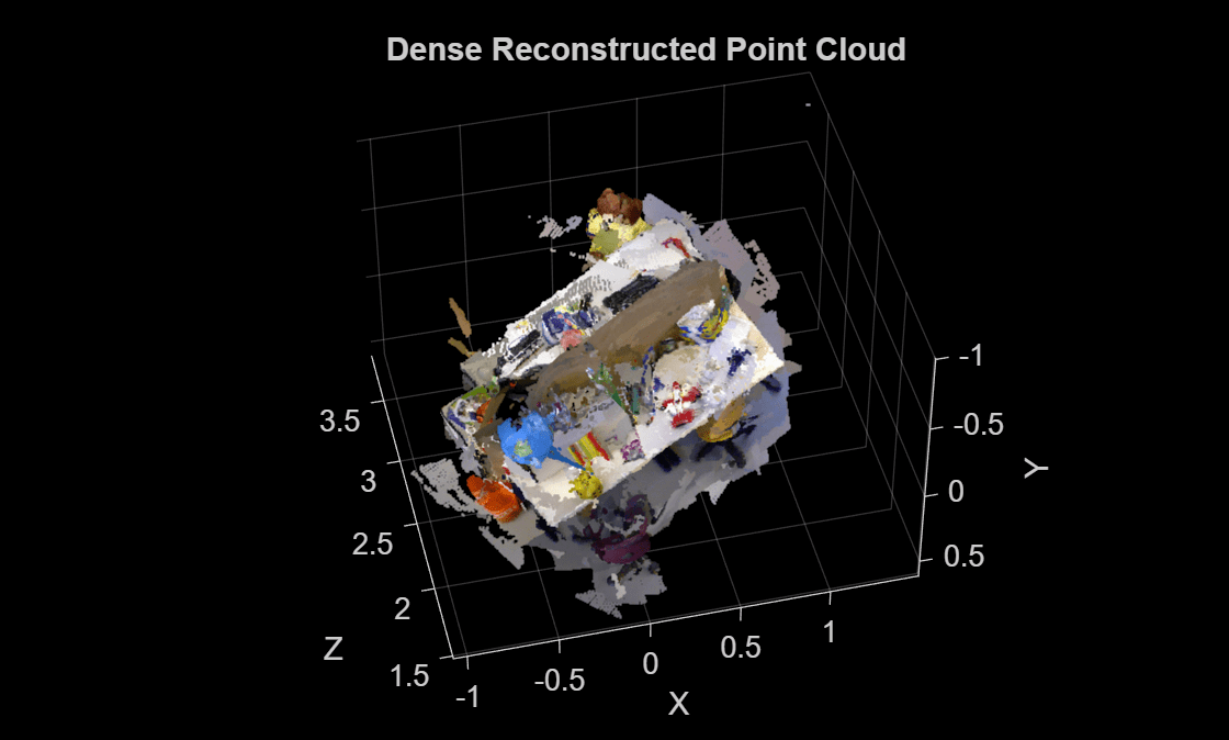
Visualize the point cloud and the camera positions of the views used in the dense reconstruction. Despite challenging camera motion and casually captured settings in this image sequence, the details of the desk and the objects on it are accurate in the reconstruction. The process used in this example discards a large number of uncertain or inconsistent depth estimates in the process, resulting in gaps in the final point cloud. These are often textureless, planar surfaces such as the floor, or distant structures such as the walls.
figure
pcshow(ptCloudsMerged, VerticalAxis="y", VerticalAxisDir="down");
xlabel("X")
ylabel("Y")
zlabel("Z")
title("Dense Reconstructed Point Cloud")
The example demonstrates a simplified version of dense reconstruction, relying on robust estimates of optical flow, camera pose estimation and sparse reconstruction results from Structure-from-Motion. See Schönberger et al. [1] for more details on rigorous multi-view stereo methods for dense reconstruction. For higher fidelity reconstruction, you can consider using additional sensors such as RGB-D or stereo cameras, capturing the data at high resolution and avoiding motion blur, or by using deep learning techniques such as the nerfacto Neural Radiance Field (NeRF) model. For more information, see Reconstruct 3-D Scenes and Synthesize Novel Views Using Neural Radiance Field Model.
References
[1] J. L. Schönberger, E. Zheng, M. Pollefeys, and J.-M. Frahm, "Pixelwise View Selection for Unstructured Multi-View Stereo," in Proceedings of the European Conference on Computer Vision (ECCV), 2016.
[2] Teed, Zachary, and Jia Deng. "RAFT: Recurrent All-Pairs Field Transforms for Optical Flow," in Proceedings of the European Conference on Computer Vision (ECCV), 2020.
[3] Sturm, Jürgen, Nikolas Engelhard, Felix Endres, Wolfram Burgard, and Daniel Cremers. "A benchmark for the evaluation of RGB-D SLAM systems". In Proceedings of IEEE/RSJ International Conference on Intelligent Robots and Systems, pp. 573-580, 2012.