Vehicle Lateral Acceleration at Different Speeds
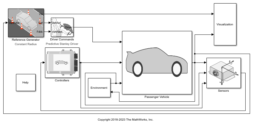
This example shows how to use the vehicle dynamics constant radius reference application to analyze the impact of speed on the vehicle lateral dynamics. Specifically, you can examine the lateral acceleration when you run the maneuver with different speeds. For information about similar maneuvers, see standards SAE J266_199601 and ISO 4138:2012.
During the maneuver, the vehicle uses a predictive driver model to maintain a pre-specified turn radius at a set velocity.
For more information about the reference application, see Constant Radius Maneuver.
vdynblksConstRadiusStart;
Run a Constant Radius Maneuver
1. Open the Reference Generator block. By default, the maneuver is set with these parameters:
Maneuver —
Constant radiusUse maneuver-specific driver, initial position, and scene — on
Longitudinal velocity reference — 35 mph
Radius value — 100 m
2. Select the Reference Generator block 3D Engine tab. By default, the 3D Engine parameter is Disabled. Simulating models in the 3D visualization environment requires Simulink® 3D Animation™. For the 3D visualization engine platform requirements and hardware recommendations, see the Unreal Engine Simulation Environment Requirements and Limitations.
3. Run the maneuver with the default settings. As the simulation runs, view the vehicle information.
mdl = 'CRReferenceApplication';
sim(mdl);
### Searching for referenced models in model 'CRReferenceApplication'.
### Total of 3 models to build.
### Starting serial model build.
### Successfully updated the model reference simulation target for: Driveline
### Successfully updated the model reference simulation target for: PassVeh14DOF
### Successfully updated the model reference simulation target for: SiMappedEngineV

Build Summary

Model reference simulation targets:

Model            Build Reason                                        Status                        Build Duration
=================================================================================================================
Driveline        Target (Driveline_msf.mexw64) did not exist.        Code generated and compiled.  0h 1m 28.309s
PassVeh14DOF     Target (PassVeh14DOF_msf.mexw64) did not exist.     Code generated and compiled.  0h 3m 27.485s
SiMappedEngineV  Target (SiMappedEngineV_msf.mexw64) did not exist.  Code generated and compiled.  0h 0m 26.268s

3 of 3 models built (0 models already up to date)
Build duration: 0h 6m 4.3413s
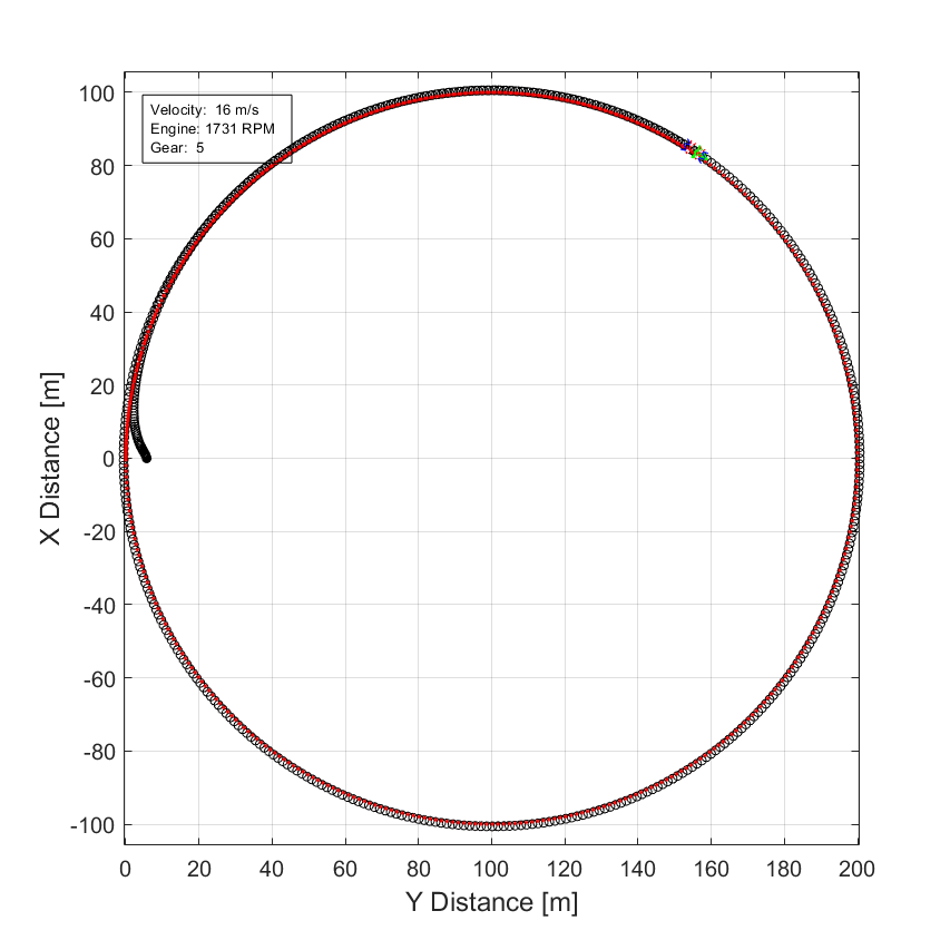
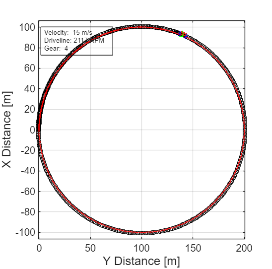
In the Vehicle Position window, view the vehicle longitudinal distance as a function or the lateral distance. The yellow line displays the yaw rate. The blue line shows the steering angle.
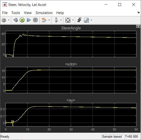
In the Visualization subsystem, open the Steer, Velocity, Lat Accel Scope block to display the steering angle, velocity, and lateral acceleration versus time.
Sweep Speed
Run the constant radius reference application with three different speeds. Stop the simulation if the vehicle exceeds a lateral acceleration threshold of 0.5 g.
1. In the constant radius reference application model CRReferenceApplication, open the Reference Generator block. The Longitudinal speed set point, xdot_r block parameter sets the vehicle speed. By default, the speed is 35 mph.
2. Enable signal logging for the velocity, lane, and ISO signals. You can use the Simulink® editor or, alternatively, these MATLAB® commands. Save the model.
Select the Reference Generator block Stop simulation at lateral acceleration threshold parameter.
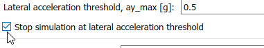
set_param([mdl '/Reference Generator'],'cr_ay_stop','on');
Enable signal logging for the Reference Generator Vis signal outport.
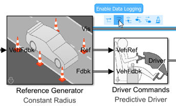
ph=get_param('CRReferenceApplication/Reference Generator','PortHandles');
set_param(ph.Outport(1),'DataLogging','on');
Enable signal logging for the Passenger Vehicle block outport signal.
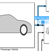
ph=get_param('CRReferenceApplication/Passenger Vehicle','PortHandles');
set_param(ph.Outport(1),'DataLogging','on');
In the Visualization subsystem, enable signal logging for the ISO block.
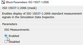
set_param([mdl '/Visualization/ISO 15037-1:2006'],'Measurement','Enable');
3. Set up a speed set point vector, vmax, that you want to investigate. For example, at the command line, type:
vmax = [32, 35, 38];
numExperiments = length(vmax);

4. Create an array of simulation inputs that set the Reference Generator block parameter Longitudinal velocity reference, xdot_r equal to vmax.
for idx = numExperiments:-1:1
    in(idx) = Simulink.SimulationInput(mdl);
    in(idx) = in(idx).setBlockParameter([mdl '/Reference Generator'], ...
        'xdot_r', num2str(vmax(idx)));
end

5. Save the model and run the simulations.
save_system(mdl)
tic;
simout = parsim(in,'ShowSimulationManager','on');
toc;
[21-Jan-2026 12:17:41] Checking for availability of parallel pool...
Starting parallel pool (parpool) using the 'Processes' profile ...
21-Jan-2026 12:18:55: Job Queued. Waiting for parallel pool job with ID 1 to start ...
Connected to parallel pool with 10 workers.
[21-Jan-2026 12:20:23] Starting Simulink on parallel workers...
[21-Jan-2026 12:21:33] Loading project on parallel workers...
[21-Jan-2026 12:21:33] Configuring simulation cache folder on parallel workers...
[21-Jan-2026 12:21:59] Loading model on parallel workers...
[21-Jan-2026 12:23:50] Running simulations...
[21-Jan-2026 12:27:22] Completed 1 of 3 simulation runs
[21-Jan-2026 12:27:22] Received simulation output (size: 23.57 MB) for run 2 from parallel worker.
[21-Jan-2026 12:27:23] Completed 2 of 3 simulation runs
[21-Jan-2026 12:27:23] Received simulation output (size: 23.49 MB) for run 1 from parallel worker.
[21-Jan-2026 12:27:23] Completed 3 of 3 simulation runs
[21-Jan-2026 12:27:23] Received simulation output (size: 23.69 MB) for run 3 from parallel worker.
[21-Jan-2026 12:27:24] Cleaning up parallel workers...
Elapsed time is 612.647536 seconds.

6. Close the Simulation Data Inspector windows.
Use Simulation Data Inspector to Analyze Results
Use the Simulation Data Inspector to examine the results. You can use the UI or, alternatively, command-line functions.
1. Open the Simulation Data Inspector. On the Simulink Toolstrip, on the Simulation tab, under Review Results, click Data Inspector.
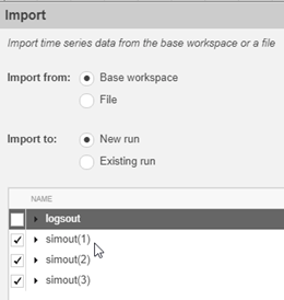
In the Simulation Data Inspector, select Import.
In the Import dialog box, clear logsout. Select
simout(1),simout(2), andsimout(3). Select Import.
Use the Simulation Data Inspector to examine the results.
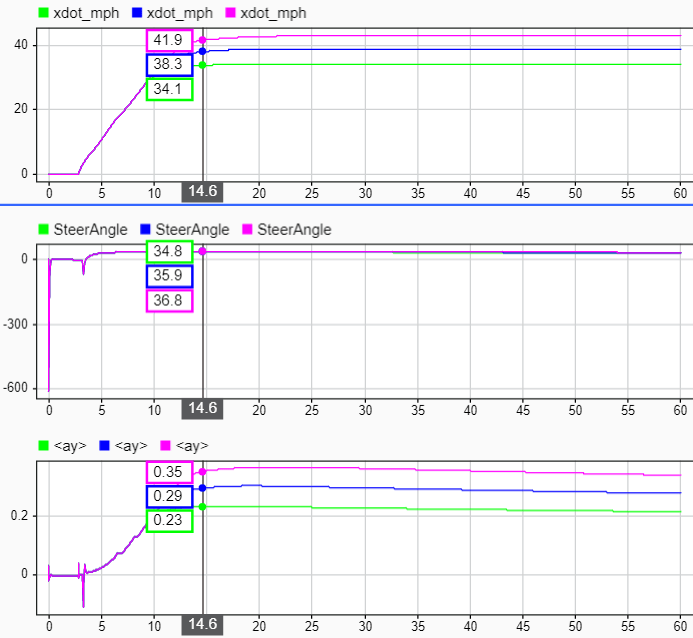
2. Alternatively, use these MATLAB commands to plot the longitudinal velocity, lateral acceleration, and the steering wheel angle.
for idx = 1:numExperiments
    % Create sdi run object
    simoutRun(idx)=Simulink.sdi.Run.create;
    simoutRun(idx).Name=['Velocity = ', num2str(vmax(idx))];
    add(simoutRun(idx),'vars',simout(idx));
end
sigcolor=[0 1 0;0 0 1;1 0 1];
for idx = 1:numExperiments
    % Extract the lateral acceleration, position, and steering
    msignal(idx)=getSignalsByName(simoutRun(idx), 'xdot_mph');
    msignal(idx).LineColor =sigcolor((idx),:);
    ssignal(idx)=getSignalsByName(simoutRun(idx), 'SteerAngle');
    ssignal(idx).LineColor =sigcolor((idx),:);
    asignal(idx)=getSignalsByName(simoutRun(idx), 'ay');
    asignal(idx).LineColor =sigcolor((idx),:);
end
Simulink.sdi.view
Simulink.sdi.setSubPlotLayout(3,1);
for idx = 1:numExperiments
    % Plot the lateral position, steering angle, and lateral acceleration
    plotOnSubPlot(msignal(idx),1,1,true);
    plotOnSubPlot(ssignal(idx),2,1,true);
    plotOnSubPlot(asignal(idx),3,1,true);
end
The results are similar to these plots, which indicate that the greatest lateral acceleration occurs when the vehicle velocity is 45 mph.
Further Analysis
To explore the results further, use these commands to extract the lateral acceleration, steering angle, and vehicle trajectory from the simout object.
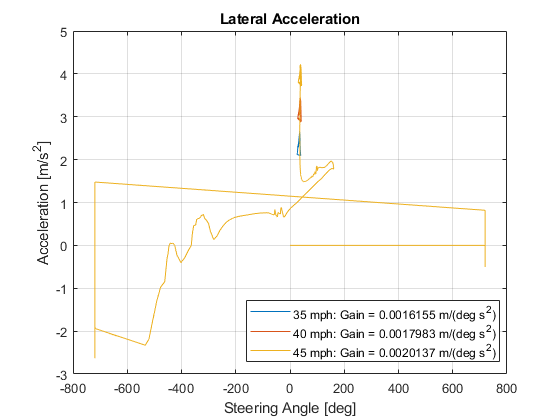
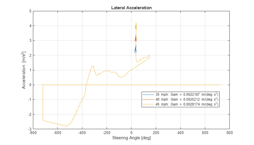
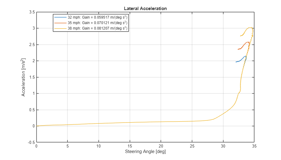
1. Extract the lateral acceleration and steering angle. Plot the data. The results are similar to this plot.
figure
for idx = 1:numExperiments
    % Extract Data
    log = get(simout(idx),'logsout');
    sa=log.get('Steering-wheel angle').Values;
    ay=log.get('Lateral acceleration').Values;
    firstorderfit = polyfit(sa.Data,ay.Data,1);
    gain(idx)=firstorderfit(1);
    legend_labels{idx} = [num2str(vmax(idx)), ' mph: Gain = ', ...
        num2str(gain(idx)), ' m/(deg s^2)'];
    % Plot steering angle vs. lateral acceleration
    plot(sa.Data,ay.Data)
    hold on
end
% Add labels to the plots
legend(legend_labels, 'Location', 'best');
title('Lateral Acceleration')
xlabel('Steering Angle [deg]')
ylabel('Acceleration [m/s^2]')
grid on

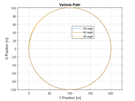
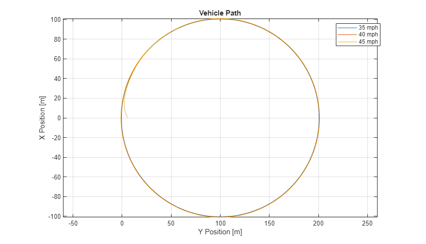
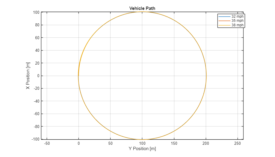
2. Extract the vehicle path. Plot the data. The results are similar to this plot.
figure
for idx = 1:numExperiments
    % Extract Data
    log = get(simout(idx),'logsout');
    xValues = getSignalsByName(simoutRun(idx), 'Passenger Vehicle:1.Body.InertFrm.Cg.Disp.X').Values;
    yValues = getSignalsByName(simoutRun(idx), 'Passenger Vehicle:1.Body.InertFrm.Cg.Disp.Y').Values;
    x = xValues.Data;
    y = yValues.Data;
    legend_labels{idx} = [num2str(vmax(idx)), ' mph'];
    % Plot vehicle location
    axis('equal')
    plot(y,x)
    hold on
end
% Add labels to the plots
legend(legend_labels, 'Location', 'best');
title('Vehicle Path')
xlabel('Y Position [m]')
ylabel('X Position [m]')
grid on
References
[1] J266_199601. Steady-State Directional Control Test Procedures for Passenger Cars and Light Trucks. Warrendale, PA: SAE International, 1996.
[2] ISO 4138:2012. Passenger cars -- Steady-state circular driving behaviour -- Open-loop test methods. ISO (International Organization for Standardization), 2012.
See Also
Simulink.SimulationInput | Simulink.SimulationOutput | polyfit