taylor
Taylor series
Description
T = taylor(f,var)f with the Taylor series expansion of f up to the fifth order
at the point var = 0. If you do not specify
var, then taylor uses the default
variable determined by symvar(f,1).
T = taylor(___,Name=Value)
Examples
Find the Maclaurin series expansions of the exponential, sine, and cosine functions up to the fifth order.
syms x
T1 = taylor(exp(x))
T1 =
T2 = taylor(sin(x))
T2 =
T3 = taylor(cos(x))
T3 =
You can use the sympref function to modify the output order of symbolic polynomials. Redisplay the polynomials in ascending order.
sympref("PolynomialDisplayStyle","ascend");
T1
T1 =
T2
T2 =
T3
T3 =
The display format you set using sympref persists through your current and future MATLAB® sessions. Restore the default value by specifying the "default" option.
sympref("default");Find the Taylor series expansions at for these functions. The default expansion point is 0. To specify a different expansion point, use ExpansionPoint.
syms x
T = taylor(log(x),x,ExpansionPoint=1)
T =
Alternatively, specify the expansion point as the third argument of taylor.
T = taylor(acot(x),x,1)
T =
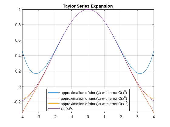
Find the Maclaurin series expansion for f = sin(x)/x. The default truncation order is 6. The Taylor series approximation of this expression does not have a fifth-degree term, so taylor approximates this expression with the fourth-degree polynomial.
syms x
f = sin(x)/x;
T6 = taylor(f,x);
Use Order to control the truncation order. For example, approximate the same expression up to the orders 7 and 9.
T8 = taylor(f,x,Order=8);
T10 = taylor(f,x,Order=10);
Plot the original expression f and its approximations T6, T8, and T10. Note how the accuracy of the approximation depends on the truncation order.
fplot([T6 T8 T10 f])
xlim([-4 4])
grid on
legend("approximation of sin(x)/x with error O(x^6)", ...
       "approximation of sin(x)/x with error O(x^8)", ...
       "approximation of sin(x)/x with error O(x^{10})", ...
       "sin(x)/x",Location="Best")
title("Taylor Series Expansion")
Find the Taylor series expansion of this expression. By default, taylor uses an absolute order, which is the truncation order of the computed series.
syms x
T = taylor(1/exp(x) - exp(x) + 2*x,x,Order=5)
T =
Find the Taylor series expansion with a relative truncation order by using OrderMode. For some expressions, a relative truncation order provides more accurate approximations.
T = taylor(1/exp(x) - exp(x) + 2*x,x,Order=5,OrderMode="relative")T =
Find the Maclaurin series expansion of this multivariate expression. If you do not specify the vector of variables, taylor treats f as a function of one independent variable.
syms x y z
f = sin(x) + cos(y) + exp(z);
T = taylor(f)
T =
Find the multivariate Maclaurin series expansion by specifying the vector of variables.
syms x y z
f = sin(x) + cos(y) + exp(z);
T = taylor(f,[x,y,z])
T =
You can use the sympref function to modify the output order of a symbolic polynomial. Redisplay the polynomial in ascending order.
sympref("PolynomialDisplayStyle","ascend");
T
T =
The display format you set using sympref persists through your current and future MATLAB sessions. Restore the default value by specifying the "default" option.
sympref("default");Find the multivariate Taylor series expansion by specifying both the vector of variables and the vector of values defining the expansion point.
syms x y
f = y*exp(x - 1) - x*log(y);
T = taylor(f,[x y],[1 1],Order=3)
T =
If you specify the expansion point as a scalar a, taylor transforms that scalar into a vector of the same length as the vector of variables. All elements of the expansion vector equal a.
T = taylor(f,[x y],1,Order=3)
T =
Find the error estimate when approximating a function using the Taylor series expansion. Here, consider the Taylor approximation up to the 7th order (with the truncation order ) at the expansion point .
The error or remainder in the Taylor approximation is given by the Lagrange form:
The upper bound of the error estimate can be calculated by finding a positive real number such that for all between and .
Find the Taylor series expansion of the function up to the 7th order by specifying Order as 8.
syms x
f = log(x+1)
f =
T = taylor(f,Order=8)
T =
To estimate the error in the Taylor approximation, first compute the term .
syms c
fn(c) = subs(diff(f,8),x,c)
fn(c) =
For positive values of , the upper bound of the error estimate can be calculated by using the relation (because must be a positive value between and a positive ). Next, find the upper bound of the error estimate Rupper(x) by using the Lagrange from and the relation .
Rupper(x) = 5040*x^8/factorial(8)
Rupper(x) =
Evaluate the Taylor series expansion at the point . Find the upper bound of the error estimate in the Taylor approximation.
Teval = subs(T,x,0.5)
Teval =
Rmax = double(Rupper(0.5))
Rmax =
4.8828e-04
For comparison, evaluate the exact function at and find the remainder in the Taylor approximation.
feval = subs(f,x,0.5)
feval =
R = double(abs(feval-Teval))
R =
3.3846e-04
Input Arguments
Name-Value Arguments
More About
Tips
If you use both the third argument
aandExpansionPointto specify the expansion point, then the value specified byExpansionPointprevails.If
varis a vector, then the expansion pointamust be a scalar or a vector of the same length asvar. Ifvaris a vector andais a scalar, thenais expanded into a vector of the same length asvarwith all elements equal toa.If the expansion point is infinity or negative infinity, then
taylorcomputes the Laurent series expansion, which is a power series in1/var.You can use the
sympreffunction to modify the output order of symbolic polynomials.If
taylorcannot find the Taylor series expansion, then useseriesto find the more general Puiseux series expansion.
Version History
Introduced before R2006a