acot

Symbolic inverse cotangent function

Syntax

acot(X)

Description

acot(X) returns the inverse cotangent function (arccotangent function) of X. All angles are in radians.

• For real values of X, acot(X) returns values in the interval [-pi/2,pi/2].

• For complex values of X, acot(X) returns complex values with the real parts in the interval [-pi/2,pi/2].

Examples

Inverse Cotangent Function for Numeric and Symbolic Arguments

Depending on its arguments, acot returns floating-point or exact symbolic results.

Compute the inverse cotangent function for these numbers. Because these numbers are not symbolic objects, acot returns floating-point results.

A = acot([-1, -1/3, -1/sqrt(3), 1/2, 1, sqrt(3)])

A =
   -0.7854   -1.2490   -1.0472    1.1071    0.7854    0.5236

Compute the inverse cotangent function for the numbers converted to symbolic objects. For many symbolic (exact) numbers, acot returns unresolved symbolic calls.

symA = acot(sym([-1, -1/3, -1/sqrt(3), 1/2, 1, sqrt(3)]))

symA =
[ -pi/4, -acot(1/3), -pi/3, acot(1/2), pi/4, pi/6]

Use vpa to approximate symbolic results with floating-point numbers:

vpa(symA)

ans =
[ -0.78539816339744830961566084581988,...
-1.2490457723982544258299170772811,...
-1.0471975511965977461542144610932,...
1.1071487177940905030170654601785,...
0.78539816339744830961566084581988,...
0.52359877559829887307710723054658]

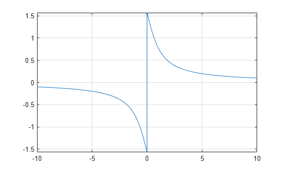
Plot Inverse Cotangent Function

Plot the inverse cotangent function on the interval from -10 to 10.

syms x
fplot(acot(x),[-10 10])
grid on

Handle Expressions Containing Inverse Cotangent Function

Many functions, such as diff, int, taylor, and rewrite, can handle expressions containing acot.

Find the first and second derivatives of the inverse cotangent function:

syms x
diff(acot(x), x)
diff(acot(x), x, x)

ans =
-1/(x^2 + 1)
 
ans =
(2*x)/(x^2 + 1)^2

Find the indefinite integral of the inverse cotangent function:

int(acot(x), x)

ans =
log(x^2 + 1)/2 + x*acot(x)

Find the Taylor series expansion of acot(x) for x > 0:

assume(x > 0)
taylor(acot(x), x)

ans =
- x^5/5 + x^3/3 - x + pi/2

For further computations, clear the assumption on x by recreating it using syms:

syms x

Rewrite the inverse cotangent function in terms of the natural logarithm:

rewrite(acot(x), 'log')

ans =
(log(1 - 1i/x)*1i)/2 - (log(1i/x + 1)*1i)/2

Input Arguments

X — Input

symbolic number | symbolic variable | symbolic expression | symbolic function | symbolic vector | symbolic matrix

Input, specified as a symbolic number, variable, expression, or function, or as a vector or matrix of symbolic numbers, variables, expressions, or functions.

Version History

Introduced before R2006a