Robust Feature Selection Using NCA for Regression
Perform feature selection that is robust to outliers using a custom robust loss function in NCA.
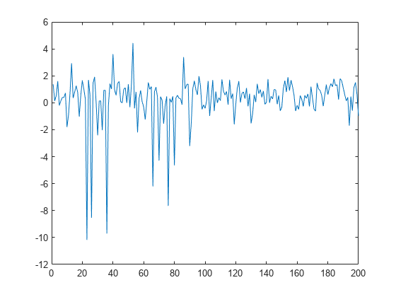
Generate data with outliers
Generate sample data for regression where the response depends on three of the predictors, namely predictors 4, 7, and 13.
rng(123,'twister') % For reproducibility
n = 200;
X = randn(n,20);
y = cos(X(:,7)) + sin(X(:,4).*X(:,13)) + 0.1*randn(n,1);
Add outliers to data.
numoutliers = 25;
outlieridx = floor(linspace(10,90,numoutliers));
y(outlieridx) = 5*randn(numoutliers,1);
Plot the data.
figure
plot(y)
Use non-robust loss function
The performance of the feature selection algorithm highly depends on the value of the regularization parameter. A good practice is to tune the regularization parameter for the best value to use in feature selection. Tune the regularization parameter using five-fold cross validation. Use the mean squared error (MSE):
First, partition the data into five folds. In each fold, the software uses 4/5th of the data for training and 1/5th of the data for validation (testing).
cvp = cvpartition(length(y),'kfold',5);
numtestsets = cvp.NumTestSets;
Compute the lambda values to test for and create an array to store the loss values.
lambdavals = linspace(0,3,50)*std(y)/length(y);
lossvals = zeros(length(lambdavals),numtestsets);
Perform NCA and compute the loss for each value and each fold.
for i = 1:length(lambdavals)
    for k = 1:numtestsets
        Xtrain = X(cvp.training(k),:);
        ytrain = y(cvp.training(k),:);
        Xtest = X(cvp.test(k),:);
        ytest = y(cvp.test(k),:);

        nca = fsrnca(Xtrain,ytrain,'FitMethod','exact', ...
            'Solver','lbfgs','Verbose',0,'Lambda',lambdavals(i), ...
            'LossFunction','mse');

        lossvals(i,k) = loss(nca,Xtest,ytest,'LossFunction','mse');
    end
end
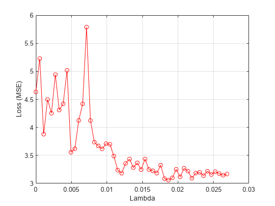
Plot the mean loss corresponding to each lambda value.
figure
meanloss = mean(lossvals,2);
plot(lambdavals,meanloss,'ro-')
xlabel('Lambda')
ylabel('Loss (MSE)')
grid on
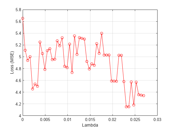
Find the value that produces the minimum average loss.
[~,idx] = min(mean(lossvals,2));
bestlambda = lambdavals(idx)
bestlambda =
0.0231
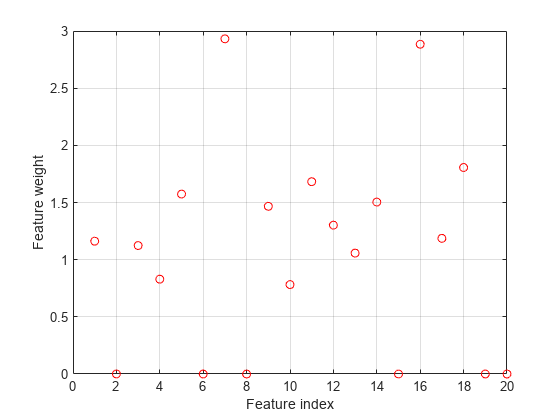
Perform feature selection using the best value and MSE.
nca = fsrnca(X,y,'FitMethod','exact','Solver','lbfgs', ...
    'Verbose',1,'Lambda',bestlambda,'LossFunction','mse');
 o Solver = LBFGS, HessianHistorySize = 15, LineSearchMethod = weakwolfe

|====================================================================================================|
|   ITER   |   FUN VALUE   |  NORM GRAD  |  NORM STEP  |  CURV  |    GAMMA    |    ALPHA    | ACCEPT |
|====================================================================================================|
|        0 |  6.414642e+00 |   8.430e-01 |   0.000e+00 |        |   7.117e-01 |   0.000e+00 |   YES  |
|        1 |  6.066100e+00 |   9.952e-01 |   1.264e+00 |    OK  |   3.741e-01 |   1.000e+00 |   YES  |
|        2 |  5.498221e+00 |   4.267e-01 |   4.250e-01 |    OK  |   4.016e-01 |   1.000e+00 |   YES  |
|        3 |  5.108548e+00 |   3.933e-01 |   8.564e-01 |    OK  |   3.599e-01 |   1.000e+00 |   YES  |
|        4 |  4.808456e+00 |   2.505e-01 |   9.352e-01 |    OK  |   8.798e-01 |   1.000e+00 |   YES  |
|        5 |  4.677382e+00 |   2.085e-01 |   6.014e-01 |    OK  |   1.052e+00 |   1.000e+00 |   YES  |
|        6 |  4.487789e+00 |   4.726e-01 |   7.374e-01 |    OK  |   5.593e-01 |   1.000e+00 |   YES  |
|        7 |  4.310099e+00 |   2.484e-01 |   4.253e-01 |    OK  |   3.367e-01 |   1.000e+00 |   YES  |
|        8 |  4.258539e+00 |   3.629e-01 |   4.521e-01 |    OK  |   4.705e-01 |   5.000e-01 |   YES  |
|        9 |  4.175345e+00 |   1.972e-01 |   2.608e-01 |    OK  |   4.018e-01 |   1.000e+00 |   YES  |
|       10 |  4.122340e+00 |   9.169e-02 |   2.947e-01 |    OK  |   3.487e-01 |   1.000e+00 |   YES  |
|       11 |  4.095525e+00 |   9.798e-02 |   2.529e-01 |    OK  |   1.188e+00 |   1.000e+00 |   YES  |
|       12 |  4.059690e+00 |   1.584e-01 |   5.213e-01 |    OK  |   9.930e-01 |   1.000e+00 |   YES  |
|       13 |  4.029208e+00 |   7.411e-02 |   2.076e-01 |    OK  |   4.886e-01 |   1.000e+00 |   YES  |
|       14 |  4.016358e+00 |   1.068e-01 |   2.696e-01 |    OK  |   6.919e-01 |   1.000e+00 |   YES  |
|       15 |  4.004521e+00 |   5.434e-02 |   1.136e-01 |    OK  |   5.647e-01 |   1.000e+00 |   YES  |
|       16 |  3.986929e+00 |   6.158e-02 |   2.993e-01 |    OK  |   1.353e+00 |   1.000e+00 |   YES  |
|       17 |  3.976342e+00 |   4.966e-02 |   2.213e-01 |    OK  |   7.668e-01 |   1.000e+00 |   YES  |
|       18 |  3.966646e+00 |   5.458e-02 |   2.529e-01 |    OK  |   1.988e+00 |   1.000e+00 |   YES  |
|       19 |  3.959586e+00 |   1.046e-01 |   4.169e-01 |    OK  |   1.858e+00 |   1.000e+00 |   YES  |

|====================================================================================================|
|   ITER   |   FUN VALUE   |  NORM GRAD  |  NORM STEP  |  CURV  |    GAMMA    |    ALPHA    | ACCEPT |
|====================================================================================================|
|       20 |  3.953759e+00 |   8.248e-02 |   2.892e-01 |    OK  |   1.040e+00 |   1.000e+00 |   YES  |
|       21 |  3.945475e+00 |   3.119e-02 |   1.698e-01 |    OK  |   1.095e+00 |   1.000e+00 |   YES  |
|       22 |  3.941567e+00 |   2.350e-02 |   1.293e-01 |    OK  |   1.117e+00 |   1.000e+00 |   YES  |
|       23 |  3.939468e+00 |   1.296e-02 |   1.805e-01 |    OK  |   2.287e+00 |   1.000e+00 |   YES  |
|       24 |  3.938662e+00 |   8.591e-03 |   5.955e-02 |    OK  |   1.553e+00 |   1.000e+00 |   YES  |
|       25 |  3.938239e+00 |   6.421e-03 |   5.334e-02 |    OK  |   1.102e+00 |   1.000e+00 |   YES  |
|       26 |  3.938013e+00 |   5.449e-03 |   6.773e-02 |    OK  |   2.085e+00 |   1.000e+00 |   YES  |
|       27 |  3.937896e+00 |   6.226e-03 |   3.368e-02 |    OK  |   7.541e-01 |   1.000e+00 |   YES  |
|       28 |  3.937820e+00 |   2.497e-03 |   2.397e-02 |    OK  |   7.940e-01 |   1.000e+00 |   YES  |
|       29 |  3.937791e+00 |   2.004e-03 |   1.339e-02 |    OK  |   1.863e+00 |   1.000e+00 |   YES  |
|       30 |  3.937784e+00 |   2.448e-03 |   1.265e-02 |    OK  |   9.667e-01 |   1.000e+00 |   YES  |
|       31 |  3.937778e+00 |   6.973e-04 |   2.906e-03 |    OK  |   4.672e-01 |   1.000e+00 |   YES  |
|       32 |  3.937778e+00 |   3.038e-04 |   9.502e-04 |    OK  |   1.060e+00 |   1.000e+00 |   YES  |
|       33 |  3.937777e+00 |   2.327e-04 |   1.069e-03 |    OK  |   1.597e+00 |   1.000e+00 |   YES  |
|       34 |  3.937777e+00 |   1.959e-04 |   1.537e-03 |    OK  |   4.026e+00 |   1.000e+00 |   YES  |
|       35 |  3.937777e+00 |   1.162e-04 |   1.464e-03 |    OK  |   3.418e+00 |   1.000e+00 |   YES  |
|       36 |  3.937777e+00 |   8.353e-05 |   3.660e-04 |    OK  |   7.304e-01 |   5.000e-01 |   YES  |
|       37 |  3.937777e+00 |   1.412e-05 |   1.412e-04 |    OK  |   7.842e-01 |   1.000e+00 |   YES  |
|       38 |  3.937777e+00 |   1.277e-05 |   3.808e-05 |    OK  |   1.021e+00 |   1.000e+00 |   YES  |
|       39 |  3.937777e+00 |   8.614e-06 |   3.698e-05 |    OK  |   2.561e+00 |   1.000e+00 |   YES  |

|====================================================================================================|
|   ITER   |   FUN VALUE   |  NORM GRAD  |  NORM STEP  |  CURV  |    GAMMA    |    ALPHA    | ACCEPT |
|====================================================================================================|
|       40 |  3.937777e+00 |   3.159e-06 |   5.299e-05 |    OK  |   4.331e+00 |   1.000e+00 |   YES  |
|       41 |  3.937777e+00 |   2.657e-06 |   1.080e-05 |    OK  |   7.038e-01 |   5.000e-01 |   YES  |
|       42 |  3.937777e+00 |   7.054e-07 |   7.036e-06 |    OK  |   9.519e-01 |   1.000e+00 |   YES  |

         Infinity norm of the final gradient = 7.054e-07
              Two norm of the final step     = 7.036e-06, TolX   = 1.000e-06
Relative infinity norm of the final gradient = 7.054e-07, TolFun = 1.000e-06
EXIT: Local minimum found.
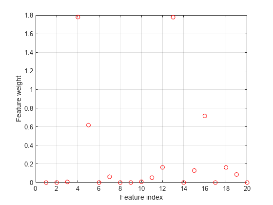
Plot selected features.
figure
plot(nca.FeatureWeights,'ro')
grid on
xlabel('Feature index')
ylabel('Feature weight')
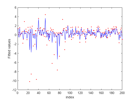
Predict the response values using the nca model and plot the fitted (predicted) response values and the actual response values.
figure
fitted = predict(nca,X);
plot(y,'r.')
hold on
plot(fitted,'b-')
xlabel('index')
ylabel('Fitted values')
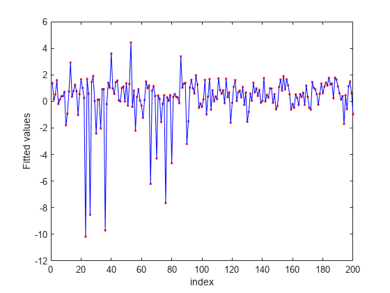
fsrnca tries to fit every point in data including the outliers. As a result it assigns nonzero weights to many features besides predictors 4, 7, and 13.
Use built-in robust loss function
Repeat the same process of tuning the regularization parameter, this time using the built-in -insensitive loss function:
-insensitive loss function is more robust to outliers than mean squared error.
lambdavals = linspace(0,3,50)*std(y)/length(y);
cvp = cvpartition(length(y),'kfold',5);
numtestsets = cvp.NumTestSets;
lossvals = zeros(length(lambdavals),numtestsets);

for i = 1:length(lambdavals)
    for k = 1:numtestsets
        Xtrain = X(cvp.training(k),:);
        ytrain = y(cvp.training(k),:);
        Xtest = X(cvp.test(k),:);
        ytest = y(cvp.test(k),:);

        nca = fsrnca(Xtrain,ytrain,'FitMethod','exact', ...
            'Solver','sgd','Verbose',0,'Lambda',lambdavals(i), ...
            'LossFunction','epsiloninsensitive','Epsilon',0.8);

        lossvals(i,k) = loss(nca,Xtest,ytest,'LossFunction','mse');
    end
end
The value to use depends on the data and the best value can be determined using cross-validation as well. But choosing the value is out of scope of this example. The choice of in this example is mainly for illustrating the robustness of the method.
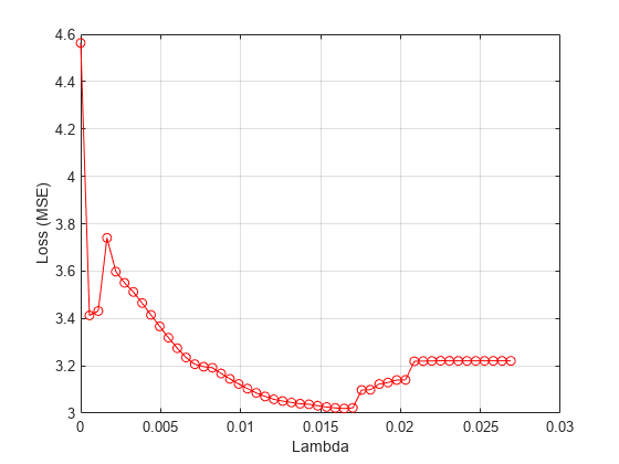
Plot the mean loss corresponding to each lambda value.
figure
meanloss = mean(lossvals,2);
plot(lambdavals,meanloss,'ro-')
xlabel('Lambda')
ylabel('Loss (MSE)')
grid on
Find the lambda value that produces the minimum average loss.
[~,idx] = min(mean(lossvals,2));
bestlambda = lambdavals(idx)
bestlambda =
0.0187
Fit neighborhood component analysis model using -insensitive loss function and best lambda value.
nca = fsrnca(X,y,'FitMethod','exact','Solver','sgd', ...
    'Lambda',bestlambda,'LossFunction','epsiloninsensitive','Epsilon',0.8);
Plot selected features.
figure
plot(nca.FeatureWeights,'ro')
grid on
xlabel('Feature index')
ylabel('Feature weight')
Plot fitted values.
figure
fitted = predict(nca,X);
plot(y,'r.')
hold on
plot(fitted,'b-')
xlabel('index')
ylabel('Fitted values')
-insensitive loss seems more robust to outliers. It identified fewer features than MSE as relevant. The fit shows that it is still impacted by some of the outliers.
Use custom robust loss function
Define a custom robust loss function that is robust to outliers to use in feature selection for regression:
customlossFcn = @(yi,yj) 1 - exp(-abs(yi-yj'));
Tune the regularization parameter using the custom-defined robust loss function.
lambdavals = linspace(0,3,50)*std(y)/length(y);
cvp = cvpartition(length(y),'kfold',5);
numtestsets = cvp.NumTestSets;
lossvals = zeros(length(lambdavals),numtestsets);

for i = 1:length(lambdavals)
    for k = 1:numtestsets
        Xtrain = X(cvp.training(k),:);
        ytrain = y(cvp.training(k),:);
        Xtest = X(cvp.test(k),:);
        ytest = y(cvp.test(k),:);

        nca = fsrnca(Xtrain,ytrain,'FitMethod','exact', ...
            'Solver','lbfgs','Verbose',0,'Lambda',lambdavals(i), ...
            'LossFunction',customlossFcn);

        lossvals(i,k) = loss(nca,Xtest,ytest,'LossFunction','mse');
    end
end
Plot the mean loss corresponding to each lambda value.
figure
meanloss = mean(lossvals,2);
plot(lambdavals,meanloss,'ro-')
xlabel('Lambda')
ylabel('Loss (MSE)')
grid on
Find the value that produces the minimum average loss.
[~,idx] = min(mean(lossvals,2));
bestlambda = lambdavals(idx)
bestlambda =
0.0165
Perform feature selection using the custom robust loss function and best value.
nca = fsrnca(X,y,'FitMethod','exact','Solver','lbfgs', ...
    'Verbose',1,'Lambda',bestlambda,'LossFunction',customlossFcn);
 o Solver = LBFGS, HessianHistorySize = 15, LineSearchMethod = weakwolfe

|====================================================================================================|
|   ITER   |   FUN VALUE   |  NORM GRAD  |  NORM STEP  |  CURV  |    GAMMA    |    ALPHA    | ACCEPT |
|====================================================================================================|
|        0 |  8.610073e-01 |   4.921e-02 |   0.000e+00 |        |   1.219e+01 |   0.000e+00 |   YES  |
|        1 |  6.582278e-01 |   2.328e-02 |   1.820e+00 |    OK  |   2.177e+01 |   1.000e+00 |   YES  |
|        2 |  5.706490e-01 |   2.241e-02 |   2.360e+00 |    OK  |   2.541e+01 |   1.000e+00 |   YES  |
|        3 |  5.677090e-01 |   2.666e-02 |   7.583e-01 |    OK  |   1.092e+01 |   1.000e+00 |   YES  |
|        4 |  5.620806e-01 |   5.524e-03 |   3.335e-01 |    OK  |   9.973e+00 |   1.000e+00 |   YES  |
|        5 |  5.616054e-01 |   1.428e-03 |   1.025e-01 |    OK  |   1.736e+01 |   1.000e+00 |   YES  |
|        6 |  5.614779e-01 |   4.446e-04 |   8.350e-02 |    OK  |   2.507e+01 |   1.000e+00 |   YES  |
|        7 |  5.614653e-01 |   4.118e-04 |   2.466e-02 |    OK  |   2.105e+01 |   1.000e+00 |   YES  |
|        8 |  5.614620e-01 |   1.307e-04 |   1.373e-02 |    OK  |   2.002e+01 |   1.000e+00 |   YES  |
|        9 |  5.614615e-01 |   9.318e-05 |   4.128e-03 |    OK  |   3.683e+01 |   1.000e+00 |   YES  |
|       10 |  5.614611e-01 |   4.579e-05 |   8.785e-03 |    OK  |   6.170e+01 |   1.000e+00 |   YES  |
|       11 |  5.614610e-01 |   1.232e-05 |   1.582e-03 |    OK  |   2.000e+01 |   5.000e-01 |   YES  |
|       12 |  5.614610e-01 |   3.174e-06 |   4.742e-04 |    OK  |   2.510e+01 |   1.000e+00 |   YES  |
|       13 |  5.614610e-01 |   7.896e-07 |   1.683e-04 |    OK  |   2.959e+01 |   1.000e+00 |   YES  |

         Infinity norm of the final gradient = 7.896e-07
              Two norm of the final step     = 1.683e-04, TolX   = 1.000e-06
Relative infinity norm of the final gradient = 7.896e-07, TolFun = 1.000e-06
EXIT: Local minimum found.
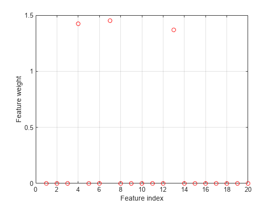
Plot selected features.
figure
plot(nca.FeatureWeights,'ro')
grid on
xlabel('Feature index')
ylabel('Feature weight')
Plot fitted values.
figure
fitted = predict(nca,X);
plot(y,'r.')
hold on
plot(fitted,'b-')
xlabel('index')
ylabel('Fitted values')
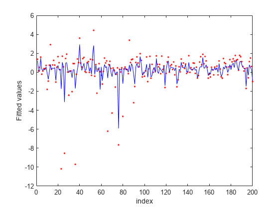
In this case, the loss is not affected by the outliers and results are based on most of the observation values. fsrnca detects the predictors 4, 7, and 13 as relevant features and does not select any other features.
Why does the loss function choice affect the results?
First, compute the loss functions for a series of values for the difference between two observations.
deltay = linspace(-10,10,1000)';
Compute custom loss function values.
customlossvals = customlossFcn(deltay,0);
Compute epsilon insensitive loss function and values.
epsinsensitive = @(yi,yj,E) max(0,abs(yi-yj')-E);
epsinsenvals = epsinsensitive(deltay,0,0.5);
Compute MSE loss function and values.
mse = @(yi,yj) (yi-yj').^2;
msevals = mse(deltay,0);
Now, plot the loss functions to see their difference and why they affect the results in the way they do.
figure
plot(deltay,customlossvals,'g-',deltay,epsinsenvals,'b-',deltay,msevals,'r-')
xlabel('(yi - yj)')
ylabel('loss(yi,yj)')
legend('customloss','epsiloninsensitive','mse')
ylim([0 20])
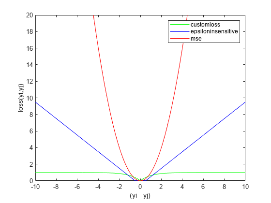
As the difference between two response values increases, MSE increases quadratically, which makes it very sensitive to outliers. As fsrnca tries to minimize this loss, it ends up identifying more features as relevant. The epsilon insensitive loss is more resistant to outliers than MSE, but eventually it does start to increase linearly as the difference between two observations increase. As the difference between two observations increase, the robust loss function does approach 1 and stays at that value even though the difference between the observations keeps increasing. Out of three, it is the most robust to outliers.
See Also
fsrnca | FeatureSelectionNCARegression | refit | predict | loss