Main Content

nlpredci

Nonlinear regression prediction confidence intervals

Description

example

[Ypred,delta] = nlpredci(modelfun,X,beta,R,'Covar',CovB) returns predictions, Ypred, and 95% confidence interval half-widths, delta, for the nonlinear regression model modelfun at input values X. Before calling nlpredci, use nlinfit to fit modelfun and get the estimated coefficients, beta, residuals, R, and variance-covariance matrix, CovB.

example

[Ypred,delta] = nlpredci(modelfun,X,beta,R,'Covar',CovB,Name,Value) uses additional options specified by one or more name-value pair arguments.

example

[Ypred,delta] = nlpredci(modelfun,X,beta,R,'Jacobian',J) returns predictions, Ypred, and 95% confidence interval half-widths, delta, for the nonlinear regression model modelfun at input values X. Before calling nlpredci, use nlinfit to fit modelfun and get the estimated coefficients, beta, residuals, R, and Jacobian, J.

If you use a robust option with nlinfit, then you should use the Covar syntax rather than the Jacobian syntax. The variance-covariance matrix, CovB, is required to properly take the robust fitting into account.

example

[Ypred,delta] = nlpredci(modelfun,X,beta,R,'Jacobian',J,Name,Value) uses additional options specified by one or more name-value pair arguments.

Examples

collapse all

Load sample data.

S = load('reaction');
X = S.reactants;
y = S.rate;
beta0 = S.beta;

Fit the Hougen-Watson model to the rate data using the initial values in beta0.

[beta,R,J] = nlinfit(X,y,@hougen,beta0);

Obtain the predicted response and 95% confidence interval half-width for the value of the curve at average reactant levels.

[ypred,delta] = nlpredci(@hougen,mean(X),beta,R,'Jacobian',J)
ypred = 5.4622
delta = 0.1921

Compute the 95% confidence interval for the value of the curve.

[ypred-delta,ypred+delta]
ans = 1×2

    5.2702    5.6543

Load sample data.

S = load('reaction');
X = S.reactants;
y = S.rate;
beta0 = S.beta;

Fit the Hougen-Watson model to the rate data using the initial values in beta0.

[beta,R,J] = nlinfit(X,y,@hougen,beta0);

Obtain the predicted response and 95% prediction interval half-width for a new observation with reactant levels [100,100,100].

[ypred,delta] = nlpredci(@hougen,[100,100,100],beta,R,'Jacobian',J,...
                         'PredOpt','observation')
ypred = 1.8346
delta = 0.5101

Compute the 95% prediction interval for the new observation.

[ypred-delta,ypred+delta]
ans = 1×2

    1.3245    2.3447

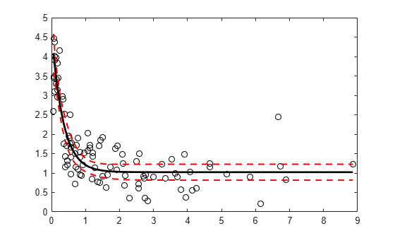
Generate sample data from the nonlinear regression model y=b1+b2exp{b3x}+ϵ, where b1, b2, and b3 are coefficients, and the error term is normally distributed with mean 0 and standard deviation 0.5.

modelfun = @(b,x)(b(1)+b(2)*exp(-b(3)*x));

rng('default') % for reproducibility
b = [1;3;2];
x = exprnd(2,100,1);
y = modelfun(b,x) + normrnd(0,0.5,100,1);

Fit the nonlinear model using robust fitting options.

opts = statset('nlinfit');
opts.RobustWgtFun = 'bisquare';
beta0 = [2;2;2];
[beta,R,J,CovB,MSE] = nlinfit(x,y,modelfun,beta0,opts);

Plot the fitted regression model and simultaneous 95% confidence bounds.

xrange = min(x):.01:max(x);
[ypred,delta] = nlpredci(modelfun,xrange,beta,R,'Covar',CovB,...
                         'MSE',MSE,'SimOpt','on');
lower = ypred - delta;
upper = ypred + delta;

figure()
plot(x,y,'ko') % observed data
hold on
plot(xrange,ypred,'k','LineWidth',2)
plot(xrange,[lower;upper],'r--','LineWidth',1.5)

Figure contains an axes object. The axes object contains 4 objects of type line. One or more of the lines displays its values using only markers

Load sample data.

S = load('reaction');
X = S.reactants;
y = S.rate;
beta0 = S.beta;

Specify a function handle for observation weights, then fit the Hougen-Watson model to the rate data using the specified observation weights function.

a = 1; b = 1;
weights = @(yhat) 1./((a + b*abs(yhat)).^2);
[beta,R,J,CovB] = nlinfit(X,y,@hougen,beta0,'Weights',weights);

Compute the 95% prediction interval for a new observation with reactant levels [100,100,100] using the observation weight function.

[ypred,delta] = nlpredci(@hougen,[100,100,100],beta,R,'Jacobian',J,...
                         'PredOpt','observation','Weights',weights);
[ypred-delta,ypred+delta]
ans = 1×2

    1.5264    2.1033

Load sample data.

S = load('reaction');
X = S.reactants;
y = S.rate;
beta0 = S.beta;

Fit the Hougen-Watson model to the rate data using the combined error variance model.

[beta,R,J,CovB,MSE,S] = nlinfit(X,y,@hougen,beta0,'ErrorModel','combined');

Compute the 95% prediction interval for a new observation with reactant levels [100,100,100] using the fitted error variance model.

[ypred,delta] = nlpredci(@hougen,[100,100,100],beta,R,'Jacobian',J,...
                         'PredOpt','observation','ErrorModelInfo',S);
[ypred-delta,ypred+delta]
ans = 1×2

    1.3245    2.3447

Input Arguments

collapse all

Nonlinear regression model function, specified as a function handle. modelfun must accept two input arguments, a coefficient vector and an array X—in that order—and return a vector of fitted response values.

For example, to specify the hougen nonlinear regression function, use the function handle @hougen.

Data Types: function_handle

Input values for predictions, specified as a matrix. nlpredci makes a prediction for the covariates in each row of X. There should be a column in X for each coefficient in the model.

Data Types: single | double

Estimated regression coefficients, specified as the vector of fitted coefficients returned by a previous call to nlinfit.

Data Types: single | double

Residuals for the fitted modelfun, specified as the vector of residuals returned by a previous call to nlinfit.

Estimated variance-covariance matrix for the fitted coefficients, beta, specified as the variance-covariance matrix returned by a previous call to nlinfit.

Estimated Jacobian of the nonlinear regression model, modelfun, specified as the Jacobian matrix returned by a previous call to nlinfit.

Name-Value Arguments

Specify optional pairs of arguments as Name1=Value1,...,NameN=ValueN, where Name is the argument name and Value is the corresponding value. Name-value arguments must appear after other arguments, but the order of the pairs does not matter.

Before R2021a, use commas to separate each name and value, and enclose Name in quotes.

Example: 'Alpha',0.1,'PredOpt','observation' specifies 90% prediction intervals for new observations.

Significance level for the confidence interval, specified as the comma-separated pair consisting of 'Alpha' and a scalar value in the range (0,1). If Alpha has value α, then nlpredci returns intervals with 100×(1–α)% confidence level.

The default confidence level is 95% (α = 0.05).

Example: 'Alpha',0.1

Data Types: single | double

Information about the error model fit, specified as the comma-separated pair consisting of 'ErrorModelInfo' and a structure returned by a previous call to nlinfit.

ErrorModelInfo only has an effect on the returned prediction interval when PredOpt has the value 'observation'. If you do not use ErrorModelInfo, then nlpredci assumes the error variance model is 'constant'.

The error model structure returned by nlinfit has the following fields:

ErrorModelChosen error model
ErrorParametersEstimated error parameters
ErrorVarianceFunction handle that accepts an N-by-p matrix, X, and returns an N-by-1 vector of error variances using the estimated error model
MSEMean squared error
ScheffeSimPredScheffé parameter for simultaneous prediction intervals when using the estimated error model
WeightFunctionLogical with value true if you used a custom weight function previously in nlinfit
FixedWeightsLogical with value true if you used fixed weights previously in nlinfit
RobustWeightFunctionLogical with value true if you used robust fitting previously in nlinfit

Mean squared error (MSE) for the fitted nonlinear regression model, specified as the comma-separated pair consisting of 'MSE' and the MSE value returned by a previous call to nlinfit.

If you use a robust option with nlinfit, then you must specify the MSE when predicting new observations to properly take the robust fitting into account. If you do not specify the MSE, then nlpredci computes the MSE from the residuals, R, and does not take the robust fitting into account.

For example, if mse is the MSE value returned by nlinfit, then you can specify 'MSE',mse.

Data Types: single | double

Prediction interval to compute, specified as the comma-separated pair consisting of 'PredOpt' and either 'curve' or 'observation'.

  • If you specify the value 'curve', then nlpredci returns confidence intervals for the estimated curve (function value) at the observations X.

  • If you specify the value 'observation', then nlpredci returns prediction intervals for new observations at X.

If you specify 'observation' after using a robust option with nlinfit, then you must also specify a value for MSE to provide the robust estimate of the mean squared error.

Example: 'PredOpt','observation'

Indicator for specifying simultaneous bounds, specified as the comma-separated pair consisting of 'SimOpt' and either 'off' or 'on'. Use the value 'off' to compute nonsimultaneous bounds, and 'on' for simultaneous bounds.

Observation weights, specified as the comma-separated pair consisting of 'Weights' and a vector of positive scalar values or a function handle. The default is no weights.

  • If you specify a vector of weights, then it must have the same number of elements as the number of observations (rows) in X.

  • If you specify a function handle for the weights, then it must accept a vector of predicted response values as input, and return a vector of real positive weights as output.

Given weights, W, nlpredci estimates the error variance at observation i by mse*(1/W(i)), where mse is the mean squared error value specified using MSE.

Example: 'Weights',@WFun

Data Types: double | single | function_handle

Output Arguments

collapse all

Predicted responses, returned as a vector with the same number of rows as X.

Confidence interval half-widths, returned as a vector with the same number of rows as X. By default, delta contains the half-widths for nonsimultaneous 95% confidence intervals for modelfun at the observations in X. You can compute the lower and upper bounds of the confidence intervals as Ypred-delta and Ypred+delta, respectively.

If 'PredOpt' has value 'observation', then delta contains the half-widths for prediction intervals of new observations at the values in X.

More About

collapse all

Confidence Intervals for Estimable Predictions

When the estimated model Jacobian is not of full rank, then it might not be possible to construct sensible confidence intervals at all prediction points. In this case, nlpredci still tries to construct confidence intervals for any estimable prediction points.

For example, suppose you fit the linear function f(xi,β)=β1xi1+β2xi2+β3xi3 at the points in the design matrix

X=(110110110101101101).

The estimated Jacobian at the values in X is the design matrix itself, J=X. Thus, the Jacobian is not of full rank:

rng('default') % For reproducibility
y = randn(6,1);

linfun = @(b,x) x*b;
beta0 = [1;1;1];
X = [repmat([1 1 0],3,1); repmat([1 0 1],3,1)];   

[beta,R,J]  = nlinfit(X,y,linfun,beta0);
Warning: The Jacobian at the solution is ill-conditioned, and
some model parameters may not be estimated well (they are not
identifiable).  Use caution in making predictions. 
> In nlinfit at 283 

In this example, nlpredci can only compute prediction intervals at points that satisfy the linear relationship

xi1=xi2+xi3.

If you try to compute confidence intervals for predictions at nonidentifiable points, nlpredci returns NaN for the corresponding interval half-widths:

xpred = [1 1 1;0 1 -1;2 1 1];
[ypred,delta] = nlpredci(linfun,xpred,beta,R,'Jacobian',J)
ypred =

   -0.0035
    0.0798
   -0.0047


delta =

       NaN
    3.8102
    3.8102
Here, the first element of delta is NaN because the first row in xpred does not satisfy the required linear dependence, and is therefore not an estimable contrast.

Tips

  • To compute confidence intervals for complex parameters or data, you need to split the problem into its real and imaginary parts. When calling nlinfit:

    1. Define your parameter vector beta as the concatenation of the real and imaginary parts of the original parameter vector.

    2. Concatenate the real and imaginary parts of the response vector Y as a single vector.

    3. Modify your model function modelfun to accept X and the purely real parameter vector, and return a concatenation of the real and imaginary parts of the fitted values.

    With the problem formulated this way, nlinfit computes real estimates, and confidence intervals are feasible.

Algorithms

  • nlpredci treats NaN values in the residuals, R, or the Jacobian, J, as missing values, and ignores the corresponding observations.

  • If the Jacobian, J, does not have full column rank, then some of the model parameters might be nonidentifiable. In this case, nlpredci tries to construct confidence intervals for estimable predictions, and returns NaN for those that are not.

References

[1] Lane, T. P. and W. H. DuMouchel. “Simultaneous Confidence Intervals in Multiple Regression.” The American Statistician. Vol. 48, No. 4, 1994, pp. 315–321.

[2] Seber, G. A. F., and C. J. Wild. Nonlinear Regression. Hoboken, NJ: Wiley-Interscience, 2003.

Version History

Introduced before R2006a