Generate Correlated Data Using Rank Correlation
Use a copula and rank correlation to generate correlated data from probability distributions that do not have an inverse cdf function available, such as the Pearson flexible distribution family.
Step 1. Generate Pearson random numbers.
Generate 1000 random numbers from two different Pearson distributions, using the pearsrnd function. The first distribution has the parameter values mu equal to 0, sigma equal to 1, skew equal to 1, and kurtosis equal to 4. The second distribution has the parameter values mu equal to 0, sigma equal to 1, skew equal to 0.75, and kurtosis equal to 3.
rng default  % For reproducibility
p1 = pearsrnd(0,1,-1,4,1000,1);
p2 = pearsrnd(0,1,0.75,3,1000,1);
At this stage, p1 and p2 are independent samples from their respective Pearson distributions, and are uncorrelated.
Step 2. Plot the Pearson random numbers.
Create a scatterhist plot to visualize the Pearson random numbers.
figure
scatterhist(p1,p2)
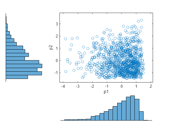
The histograms show the marginal distributions for p1 and p2. The scatterplot shows the joint distribution for p1 and p2. The lack of pattern to the scatterplot shows that p1 and p2 are independent.
Step 3. Generate random numbers using a Gaussian copula.
Use copularnd to generate 1000 correlated random numbers with a correlation coefficient equal to –0.8, using a Gaussian copula. Create a scatterhist plot to visualize the random numbers generated from the copula.
u = copularnd('Gaussian',-0.8,1000);
figure
scatterhist(u(:,1),u(:,2))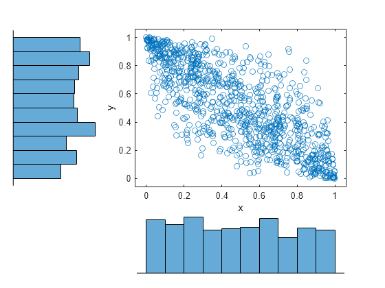
The histograms show that the data in each column of the copula have a marginal uniform distribution. The scatterplot shows that the data in the two columns are negatively correlated.
Step 4. Sort the copula random numbers.
Using Spearman's rank correlation, transform the two independent Pearson samples into correlated data.
Use the sort function to sort the copula random numbers from smallest to largest, and to return a vector of indices describing the rearranged order of the numbers.
[s1,i1] = sort(u(:,1));
[s2,i2] = sort(u(:,2));
s1 and s2 contain the numbers from the first and second columns of the copula, u, sorted in order from smallest to largest. i1 and i2 are index vectors that describe the rearranged order of the elements into s1 and s2. For example, if the first value in the sorted vector s1 is the third value in the original unsorted vector, then the first value in the index vector i1 is 3.
Step 5. Transform the Pearson samples using Spearman's rank correlation.
Create two vectors of zeros, x1 and x2, that are the same size as the sorted copula vectors, s1 and s2. Sort the values in p1 and p2 from smallest to largest. Place the values into x1 and x2, in the same order as the indices i1 and i2 generated by sorting the copula random numbers.
x1 = zeros(size(s1));
x2 = zeros(size(s2));

x1(i1) = sort(p1);
x2(i2) = sort(p2);
Step 6. Plot the correlated Pearson random numbers.
Create a scatterhist plot to visualize the correlated Pearson data.
figure
scatterhist(x1,x2)
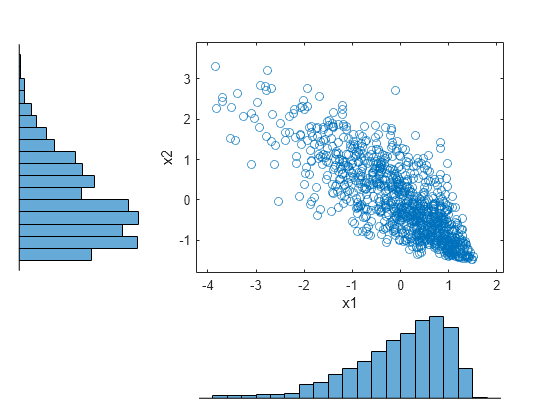
The histograms show the marginal Pearson distributions for each column of data. The scatterplot shows the joint distribution of p1 and p2, and indicates that the data are now negatively correlated.
Step 7. Confirm Spearman rank correlation coefficient values.
Confirm that the Spearman rank correlation coefficient is the same for the copula random numbers and the correlated Pearson random numbers.
copula_corr = corr(u,'Type','spearman')
copula_corr = 2×2

    1.0000   -0.7858
   -0.7858    1.0000
pearson_corr = corr([x1,x2],'Type','spearman')
pearson_corr = 2×2

    1.0000   -0.7858
   -0.7858    1.0000
The Spearman rank correlation is the same for the copula and the Pearson random numbers.