Main Content

gardnerAltmanPlot

Gardner-Altman plot for two-sample effect size

Since R2022a

    Description

    example

    gardnerAltmanPlot(X,Y) generates a Gardner-Altman plot for the mean-difference effect size of data in X and Y.

    gardnerAltmanPlot(ax,X,Y) plots into the axes with the handle ax.

    example

    gardnerAltmanPlot(___,Name=Value) specifies options using one or more name-value arguments in addition to any of the input argument combinations in previous syntaxes. For example, you can specify the type of the effect size to compute or the number of bootstrap replicas to use when computing the bootstrap confidence intervals.

    H = gardnerAltmanPlot(___) returns a graphics array H.

    Examples

    collapse all

    Load Fisher's iris data and define the variables for which to compute the median-difference effect size.

    load fisheriris
    species2 = categorical(species);
    x = meas(species2=='setosa');
    y = meas(species2=='virginica');

    Compute the median-difference effect size of the observations from two independent samples.

    effect = meanEffectSize(x,y,Effect="mediandiff")
    effect=1×2 table
                            Effect    ConfidenceIntervals
                            ______    ___________________
    
        MedianDifference     -1.5        -1.8    -1.3    


    By default, the meanEffectSize function assumes that the samples are independent (that is, Paired=false). The function uses bootstrapping to estimate the confidence intervals when the effect type is median-difference.

    Visualize the median-difference effect size using the Gardner-Altman plot.

    gardnerAltmanPlot(x,y,Effect="mediandiff");

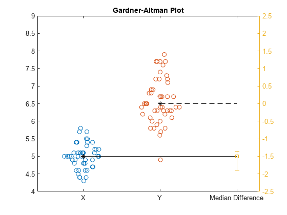
    The Gardner-Altman plot displays the two data samples on the left. The median of the sample Y corresponds to the zero effect size on the effect size axis, which is the yellow axis line on the right. The median of the sample X corresponds to the value of the effect size on the effect size axis. The plot displays the actual median-difference effect size value and the confidence intervals with the vertical error bar.

    Load Fisher's iris data and define the variables for which to compare the Cohen's d effect size.

    load fisheriris
    species2 = categorical(species);
    x = meas(species2=='setosa');
    y = meas(species2=='virginica');

    Compute the Cohen's d effect size for the observations from two independent samples, and compute the 95% confidence intervals for the effect size. By default,the meanEffectSize function uses the exact formula based on the noncentral t-distribution to estimate the confidence intervals when the effect size type is Cohen's d. Specify the bootstrapping options as follows:

    • Set meanEffectSize to use bootstrapping for confidence interval computation.

    • Use parallel computing for bootstrapping computations. You need Parallel Computing Toolbox™ for this option.

    • Use 3000 bootstrap replicas.

    rng(123) % For reproducibility
    effect = meanEffectSize(x,y,Effect="cohen",ConfidenceIntervalType="bootstrap", ...
          BootstrapOptions=statset(UseParallel=true),NumBootstraps=3000)
    Starting parallel pool (parpool) using the 'Processes' profile ...
    Connected to the parallel pool (number of workers: 6).
    
    effect=1×2 table
                   Effect     ConfidenceIntervals
                   _______    ___________________
    
        CohensD    -3.0536    -3.5621    -2.3468 


    Visualize the Cohen's d effect size using the Gardner-Altman plot with the same options set.

    gardnerAltmanPlot(x,y,Effect="cohen",ConfidenceIntervalType="bootstrap", ...
          BootstrapOptions=statset(UseParallel=true),NumBootstraps=3000);

    Figure contains an axes object. The axes object with title Gardner-Altman Plot contains 5 objects of type scatter, line, errorbar. These objects represent X, Y, X Mean, Y Mean, Cohen's d.

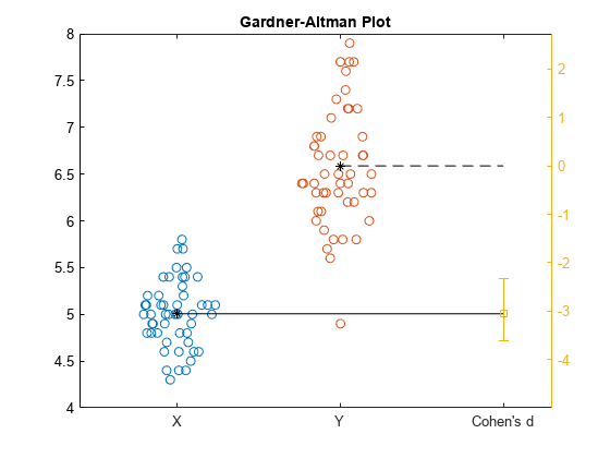
    The Gardner-Altman plot displays the two data samples on the left. The mean of the sample Y corresponds to the zero effect size on the effect size axis, which is the yellow axis line on the right. The mean of the sample X corresponds to the value of the effect size on the effect size axis. The plot displays the Cohen's d effect size value and the confidence intervals with the vertical error bar.

    Load exam grades data and define the variables to compare.

    load examgrades
    x = grades(:,1);
    y = grades(:,2);

    Compute the mean-difference effect size of the grades from the paired samples, and compute the 95% confidence intervals for the effect size.

    effect = meanEffectSize(x,y,Paired=true)
    effect=1×2 table
                           Effect     ConfidenceIntervals
                          ________    ___________________
    
        MeanDifference    0.016667    -1.3311     1.3644 


    The meanEffectSize function uses the exact method to estimate the confidence intervals when you use the mean-difference effect size.

    You can specify a different effect size type. (Note that you cannot use Glass's delta for paired samples.) Use robust Cohen's d to compare the paired sample means. Compute the 97% confidence intervals for the effect size.

    effect = meanEffectSize(x,y,Paired=true,Effect="robustcohen",Alpha=0.03)
    effect=1×2 table
                          Effect     ConfidenceIntervals
                         ________    ___________________
    
        RobustCohensD    0.059128    -0.1405    0.26573 


    The meanEffectSize function uses bootstrapping to estimate the confidence intervals when the effect size type is robust Cohen's d.

    Visualize the effect size using the Gardner-Altman plot. Specify robust Cohen's d as the effect size, and compute the 97% confidence intervals.

    gardnerAltmanPlot(x,y,Paired=true,Effect="robustcohen",Alpha=0.03);

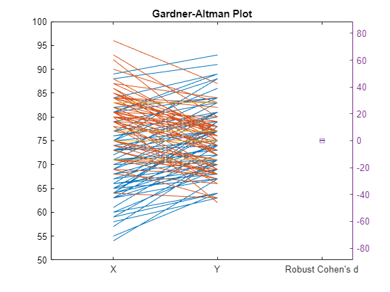
    The Gardner-Altman plot displays the paired data on the left. The blue lines show the values that are increasing and the red lines show the values that are decreasing from the first sample to the corresponding values in the paired sample, respectively. Right side of the plot displays the robust Cohen's d effect size with the 97% confidence interval.

    Input Arguments

    collapse all

    Input data, specified as a numeric vector.

    Data Types: single | double

    Input data, specified as a numeric vector.

    Data Types: single | double

    Axes for the plot, specified as an Axes or UIAxes object. If you do not specify ax, then gardnerAltmanPlot creates the plot using the current axes. For more information on creating an axes object, see axes and uiaxes.

    Name-Value Arguments

    Specify optional pairs of arguments as Name1=Value1,...,NameN=ValueN, where Name is the argument name and Value is the corresponding value. Name-value arguments must appear after other arguments, but the order of the pairs does not matter.

    Example: Effect="cliff",Alpha=0.03,ConfidenceIntervalType="bootstrap",VarianceType=unequal specifies to use the Cliff's Delta effect size, compute the 97% confidence intervals using bootstrapping, and assume the samples come from populations with unequal variances.

    Confidence level of the confidence intervals for the effect size, specified as a numeric value from 0 to 1. Default value of 0.05 corresponds to the 95% confidence level.

    Example: Alpha=0.025

    Data Types: single | double

    Options for computing bootstrap confidence intervals in parallel, specified as a structure generated by using statset("bootci"). gardnerAltmanPlot uses the following fields.

    FieldDescription
    Streams

    A RandStream object or cell array of such objects. If you do not specify Streams, gardnerAltmanPlot uses the default stream or streams. If you specify Streams, use a single object except when all of the following conditions exist:

    • You have an open parallel pool.

    • UseParallel is true.

    • UseSubstreams is false.

    In this case, use a cell array the same size as the parallel pool. If a parallel pool is not open, then Streams must supply a single random number stream.

    UseParallelThe default is false, indicating serial computation.
    UseSubstreamsSet to true to compute in a reproducible fashion. The default is false. To compute reproducibly, set Streams to a type allowing substreams: "mlfg6331_64" or "mrg32k3a".

    Computing bootstrap confidence intervals in parallel requires Parallel Computing Toolbox™.

    Example: BootstrapOptions=options

    Data Types: struct

    Type of confidence interval to compute, specified as "exact", "bootstrap", or "none". The default value is "exact" when there is an exact formula for the effect size or "bootstrap" otherwise. Specify "none" is when you do not want to compute any confidence intervals.

    The default value is "exact" for Cliff's Delta, Glass's delta, mean-difference, and Cohen's d and "bootstrap" for Kolmogorov-Smirnov statistic, median-difference, and robust Cohen's d. If you specify confidence interval type as "exact" for Kolmogorov-Smirnov statistic, median-difference, and robust Cohen's d, gardnerAltmanPlot returns an error.

    Example: ConfidenceIntervalType="none"

    Data Types: string | char

    Effect size to compute, specified as one of the following options.

    OptionDefinition
    "cohen"Cohen's d for two-sample input
    "cliff"Cliff's Delta
    "glass"

    Glass's delta; not supported by gardnerAltmanPlot for paired data

    "kstest"Kolmogorov-Smirnov statistic
    "mediandiff"Median difference
    "meandiff"Mean difference
    "robustcohen"Robust Cohen's d for two-sample input

    Example: Effect="glass"

    Data Types: string | char

    Number of bootstrap replicas to use when computing the bootstrap confidence intervals, specified as a positive integer.

    Example: NumBootstraps=1500

    Data Types: single | double

    Indicator for paired samples, specified as false or true.

    • If Paired is true, then VarianceType must be "equal".

    • If Paired is true, then Effect cannot be "glass".

    Example: Paired=true

    Data Types: logical

    Population variance assumption for two samples, specified as "equal" or "unequal". If Paired is "true", then VarianceType must be "equal".

    Example: VarianceType="unequal"

    Data Types: string | char

    Output Arguments

    collapse all

    Graphics array for the plot, returned as a 1-by-5 or 1-by-4 graphics array depending on the specified effect size and whether the data is unpaired or paired.

    • Unpaired data (Paired="false")

      • For the "meandiff", "glass", "cohen" or "robustcohen" effect size:

        H is a 1-by-5 graphics array that holds two Scatter objects, one ErrorBar object, and two Line objects.

        The Scatter objects represent the scatter plots of the input data in X and Y. The ErrorBar object represents the effect size and its confidence intervals. The Line objects represent the mean line from the control sample to the effect size and from the other sample to 0.

      • For the "mediandiff" effect size:

        H is a 1-by-5 graphics array that holds two Scatter objects, one ErrorBar object, and two Line objects that represent the median lines from the two sample data sets.

      • For the "cliff" or "kstest" effect size:

        H is a 1-by-4 graphics array that holds two Scatter objects, one ErrorBar object, and one Line object that represents the line at 0 to indicate no effect between the two groups.

    • Paired data (Paired="true")

      • H holds one to three Line objects representing the lines for the pairs that increased, decreased, or stayed the same, and one ErrorBar object representing the effect size and its confidence intervals.

    For all cases, if you choose not to generate confidence intervals for the effect (ConfidenceIntervalType="none"), the ErrorBar object is, instead, be a Line object.

    Use H to inspect and adjust the properties of the objects. To learn more about the object properties, see Scatter Properties, ErrorBar Properties, and Line Properties.

    Algorithms

    collapse all

    Effect Size

    • Cliff's Delta

      • Unpaired data

        δ=i,j=1n1,n2(xi>yj)(xi<yj)n1*n2,

        where n1 is the size of the first sample, and n2 is the size of the second sample.

      • Paired data

        gardnerAltmanPlot uses the between-group delta, which compares the differences between x and y, but excludes comparisons of paired data. For n paired samples, the result is n(n–1) comparisons [3].

    • Cohen's d

      gardnerAltmanPlot computes the unbiased estimate of Cohen's d, which is also known as Hedge's g.

      • One-sample

        d=J(df)*(x¯μ)s

      • Two-sample

        d=J(df)*(x¯y¯)s

      where df is the degrees of freedom, μ is the known population mean to compare against, s is the pooled standard deviation, and J(df) is the bias correction term. The pooled standard deviation is defined as

      s=(n11)s12+(n21)s22n1+n22,

      where n1 is the size of the first sample and n2 is the size of the second sample.

      The bias correction term are defined as

      J(df)=Γ(df/2)df/2Γ((df1)/2),

      where Γ() is the gamma function.

      Cohen's d follows a noncentral t-distribution and uses it to derive the confidence intervals. So, by default, gardnerAltmanPlot uses "exact" to compute the confidence intervals for the effect size. See [1] and [4] to see the derivation of the confidence intervals for paired versus unpaired input data.

    • Glass's Delta

      D=x¯y¯sx,

      where sx is the standard deviation of the control group. gardnerAltmanPlot uses the data in x as the control group. If you wish to use the other sample as the control group, you can swap the data in x and y and swap the sign of the test result.

      Similar to Cohen's d, Glass's delta also follows a noncentral t-distribution and uses it to derive the confidence intervals. So, by default, gardnerAltmanPlot uses "exact" to compute the confidence intervals for the effect size [4]. You cannot use this effect size for paired samples.

    • Kolmogorov-Smirnov Test Statistic

      This two-sample test statistic is the same as given in Two-Sample Kolmogorov-Smirnov Test. gardnerAltmanPlot uses bootstrapping to compute the confidence intervals.

    • Mean Difference

      • One-sample

        m=(x¯μ)

      • Two-sample

        m=(x¯y¯)

      gardnerAltmanPlot computes the confidence intervals using the t-distribution with pooled standard deviation in the two-sample case. (In the case of unequal variance assumption for two samples, the confidence intervals are called Welch-Satterthwaite confidence intervals). By default, the function uses "exact" to compute the confidence intervals for the effect size.

    • Median Difference

      M = median(x)median(y)

      gardnerAltmanPlot computes the confidence intervals using bootstrapping for the effect size.

    • Robust Cohen's d

      d=0.643*J(df)*(x¯ty¯t)sw,

      where x¯t and y¯t are the 20% trimmed means of data in x and y, respectively. sw is the pooled 20% Winsorized variance [2].

      gardnerAltmanPlot computes the confidence intervals using bootstrapping for the effect size.

    References

    [1] Cousineau, Denis, and Jean-Christophe Goulet-Pelletier. "A Study of Confidence Intervals for Cohen's d in Within-Subject Designs with New Proposals." The Quantitative Methods for Psychology 17, no. 1 (March 2021): 51--75. https://doi.org/10.20982/tqmp.17.1.p051.

    [2] Algina, James, H. J. Keselman, and R. D. Penfield. "An Alternative to Cohen's Standardized Mean Difference Effect Size: A Robust Parameter and Confidence Interval in the Two Independent Groups Case." Psychological Methods 10, no. 3 (Sept 2005): 317–28. https://doi.org/10.1037/1082-989X.10.3.317.

    [3] Hess, Melinda, and Jeffrey Kromrey. "Robust Confidence Intervals for Effect Sizes: A Comparative Study of Cohen's d and Cliff's Delta Under Non-normality and Heterogeneous Variances." Annual Meeting of the American Educational Research Association. 2004.

    [4] Delacre, Marie, Daniel Lakens, Christophe Ley, Limin Liu, and Christophe Leys. "Why Hedges G's Based on the Non-pooled Standard Deviation Should Be Reported with Welch's T-test." 2021.

    [5] Gardner, M. J., and D. G. Altman. Confidence Intervals Rather Than P Values; Estimation Rather Than Hypothesis Testing." BMJ, 292 no. 6522 (March 1986): 746–50. https://doi.org/10.1136/bmj.292.6522.746.

    Extended Capabilities

    Version History

    Introduced in R2022a