Fit Gaussian Mixture Model to Data
This example shows how to simulate data from a multivariate normal distribution, and then fit a Gaussian mixture model (GMM) to the data using fitgmdist. To create a known, or fully specified, GMM object, see Create Gaussian Mixture Model.
fitgmdist requires a matrix of data and the number of components in the GMM. To create a useful GMM, you must choose k carefully. Too few components fails to model the data accurately (i.e., underfitting to the data). Too many components leads to an over-fit model with singular covariance matrices.
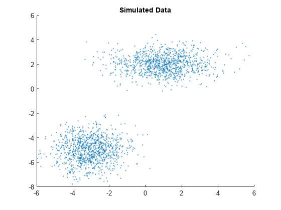
Simulate data from a mixture of two bivariate Gaussian distributions using mvnrnd.
mu1 = [1 2];
sigma1 = [2 0; 0 .5];
mu2 = [-3 -5];
sigma2 = [1 0; 0 1];
rng(1); % For reproducibility
X = [mvnrnd(mu1,sigma1,1000);
     mvnrnd(mu2,sigma2,1000)];
Plot the simulated data.
scatter(X(:,1),X(:,2),10,'.') % Scatter plot with points of size 10
title('Simulated Data')
Fit a two-component GMM. Use the 'Options' name-value pair argument to display the final output of the fitting algorithm.
options = statset('Display','final');
gm = fitgmdist(X,2,'Options',options)
5 iterations, log-likelihood = -7105.71

gm =

Gaussian mixture distribution with 2 components in 2 dimensions
Component 1:
Mixing proportion: 0.500000
Mean:   -3.0377   -4.9859

Component 2:
Mixing proportion: 0.500000
Mean:    0.9812    2.0563
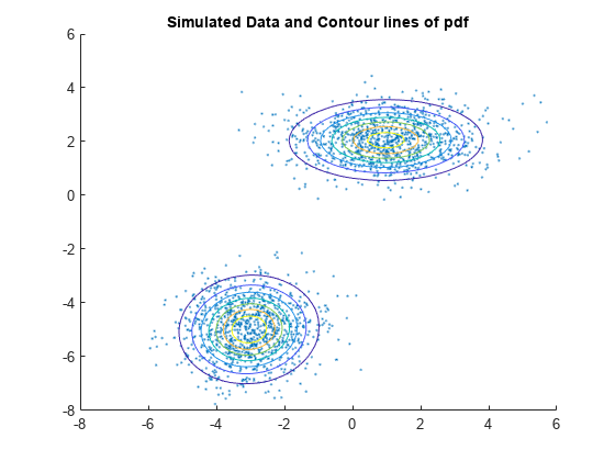
Plot the pdf of the fitted GMM.
gmPDF = @(x,y) arrayfun(@(x0,y0) pdf(gm,[x0 y0]),x,y);
hold on
h = fcontour(gmPDF,[-8 6]);
title('Simulated Data and Contour lines of pdf');
Display the estimates for means, covariances, and mixture proportions
ComponentMeans = gm.mu
ComponentMeans = 2×2

   -3.0377   -4.9859
    0.9812    2.0563
ComponentCovariances = gm.Sigma
ComponentCovariances =
ComponentCovariances(:,:,1) =

    1.0132    0.0482
    0.0482    0.9796


ComponentCovariances(:,:,2) =

    1.9919    0.0127
    0.0127    0.5533
MixtureProportions = gm.ComponentProportion
MixtureProportions = 1×2

    0.5000    0.5000
Fit four models to the data, each with an increasing number of components, and compare the Akaike Information Criterion (AIC) values.
AIC = zeros(1,4);
gm = cell(1,4);
for k = 1:4
    gm{k} = fitgmdist(X,k);
    AIC(k)= gm{k}.AIC;
end
Display the number of components that minimizes the AIC value.
[minAIC,numComponents] = min(AIC);
numComponents
numComponents =
2
The two-component model has the smallest AIC value.
Display the two-component GMM.
gm2 = gm{numComponents}gm2 = Gaussian mixture distribution with 2 components in 2 dimensions Component 1: Mixing proportion: 0.500000 Mean: -3.0377 -4.9859 Component 2: Mixing proportion: 0.500000 Mean: 0.9812 2.0563
Both the AIC and Bayesian information criteria (BIC) are likelihood-based measures of model fit that include a penalty for complexity (specifically, the number of parameters). You can use them to determine an appropriate number of components for a model when the number of components is unspecified.
See Also
fitgmdist | gmdistribution | mvnrnd | random