Main Content

capaplot

R2026b

Create process capability plot

Description

p = capaplot(x,specs) fits a normal distribution to the data x and returns the probability p that a new observation from the fitted distribution falls within the specification range given by specs. The function displays a capability plot of the fitted normal distribution function and the specification range.

example

p = capaplot(x,specs,distname) uses the continuous probability distribution distname to fit x and to compute p. (since R2026b)

example

p = capaplot(pd,specs) uses the probability distribution function information (and data, if present) in the continuous probability distribution object pd. (since R2026b)

example

p = capaplot(___,ShowHistogram=showhist) plots a histogram of the data in x (or pd, if present) in the capability plot when showhist is true, using any of the input argument combinations in the previous syntaxes. Otherwise, the capability plot displays a shaded region bounded by the specification limits and the fitted distribution function (or the distribution function in pd). (since R2026b)

example

p = capaplot(ax,___) plots into the axes specified by ax instead of the current axes (gca). (since R2024a)

[p,h] = capaplot(___) additionally returns handles to the plot elements in h.

Examples

collapse all

Simulate a sample of 100 normally-distributed measurements from a process with a mean of 3 and a standard deviation of 0.005.

x = normrnd(3,0.005,100,1);

Set a lower specification limit of 2.99 and an upper specification limit of 3.01 for the process, and then compute the capability indices and confidence intervals.

specs = [2.99 3.01];
S = capability(x,specs)
S = struct with fields:
               P: 0.9129
              Pl: 0.0339
              Pu: 0.0532
              Cp: 0.5735
            CpCI: [2×1 double]
             Cpl: 0.6088
           CplCI: [2×1 double]
             Cpu: 0.5382
           CpuCI: [2×1 double]
             Cpk: 0.5382
           CpkCI: [2×1 double]
    Distribution: 'Normal'
              mu: 3.0006
           sigma: 0.0058

The capability function fits a normal distribution to the data in x. Visualize the fitted distribution and specification limits.

p = capaplot(x,specs)
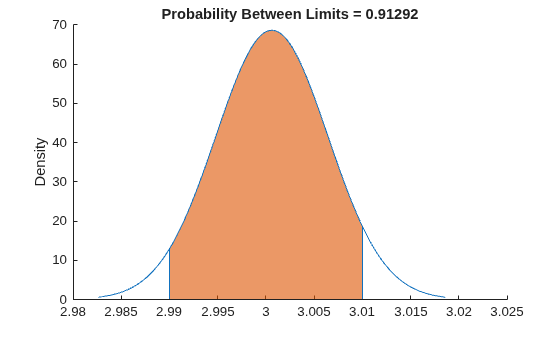
Figure contains an axes object. The axes object with title Probability Between Limits = 0.91292, ylabel Density contains 5 objects of type patch, line. This object represents Normal Distribution.

p = 
0.9129

The function also returns the probability p that a new observation from the fitted distribution lies between the specification limits, which are indicated by vertical blue lines.

Simulate a sample of 100 measurements from a Weibull distribution with the scale parameter a=10 and shape parameter b=3.

x = wblrnd(10,3,[100 1]);

Set a lower specification limit of 3 and an upper specification limit of 13 for the process, and create a capability plot using a Weibull distribution.

p = capaplot(x,[3 13],"Weibull")
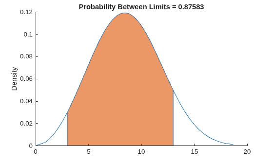
Figure contains an axes object. The axes object with title Probability Between Limits = 0.87583, ylabel Density contains 5 objects of type patch, line. This object represents Weibull Distribution.

p = 
0.8758

The function fits a Weibull distribution to the data, and displays the fit in the plot. The function also returns the probability p that a new observation from the fitted distribution lies between the specification limits, which are indicated by vertical blue lines.

Create a capability plot that displays the fit and a histogram of the data.

capaplot(x,[3 13],"Weibull",ShowHistogram=1);
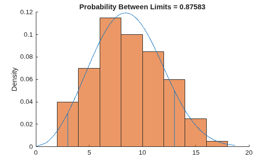
Figure contains an axes object. The axes object with title Probability Between Limits = 0.87583, ylabel Density contains 5 objects of type histogram, line. This object represents Weibull Distribution.

Simulate a sample of 100 measurements from a Rayleigh distribution with the scale parameter b=0.2.

x = raylrnd(0.2,[100 1]);

Fit a Rayleigh distribution to the sample data using the fitdist function.

pd = fitdist(x,"Rayleigh")
pd = 
  RayleighDistribution

  Rayleigh distribution
    B = 0.217169   [0.197812, 0.240759]

pd is a RayleighDistribution object that contains the fit information and the input data x.

Create a capability plot using an upper specification limit of 0.5 and no lower specification limit.

p = capaplot(pd,[-Inf 0.5])
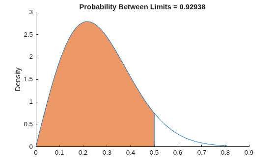
Figure contains an axes object. The axes object with title Probability Between Limits = 0.92938, ylabel Density contains 5 objects of type patch, line. This object represents Rayleigh Distribution.

p = 
0.9294

The function plots the fitted distribution function and returns the probability p that a new observation from the fitted distribution lies between the specification limits, which are indicated by vertical blue lines.

Input Arguments

collapse all

Input data, specified as a numeric vector.

Data Types: single | double

Specification limits, specified as a two-element numeric vector that contains the lower and upper specification limits. At least one element must be finite. If there is no lower specification bound, specify the first element of specs as –Inf. If there is no upper specification bound, specify the second element of specs as Inf.

Data Types: single | double

Since R2026b

Probability distribution name, specified as a character vector or string scalar containing one of the following values. distname must be the name of a continuous probability distribution supported by the fitdist function. The default value is "Normal".

You cannot specify distname when you specify pd.

ValueDescription
"Beta"Beta distribution
"BirnbaumSaunders"Birnbaum–Saunders distribution
"Burr"Burr distribution
"Exponential"Exponential distribution
"Extreme Value" or "ev"Extreme Value distribution
"Gamma"Gamma distribution
"Generalized Extreme Value" or "gev"Generalized Extreme Value distribution
"Generalized Pareto" or "gp"Generalized Pareto distribution
"Half Normal" or "hn"Half-normal distribution
"InverseGaussian"Inverse Gaussian distribution
"Kernel"Kernel distribution
"Logistic"Logistic distribution
"Loglogistic"Loglogistic distribution
"Lognormal"Lognormal distribution
"Nakagami"Nakagami distribution
"Normal" (default)Normal distribution
"Rayleigh"Rayleigh distribution
"Rician"Rician distribution
"Stable"Stable distribution
"tLocationScale"t Location-Scale distribution
"Weibull" or "wbl"Weibull distribution

Since R2026b

Probability distribution, specified as a continuous probability distribution object. The table below lists the supported probability distributions. Note that the capaplot function does not support discrete probability distribution objects.

Distribution NameDescriptionDistribution Object
"Beta"Beta distributionBetaDistribution
"BirnbaumSaunders"Birnbaum–Saunders distributionBirnbaumSaundersDistribution
"Burr"Burr distributionBurrDistribution
"Exponential"Exponential distributionExponentialDistribution
"Extreme Value" or "ev"Extreme Value distributionExtremeValueDistribution
"Gamma"Gamma distributionGammaDistribution
"Generalized Extreme Value" or "gev"Generalized Extreme Value distributionGeneralizedExtremeValueDistribution
"Generalized Pareto" or "gp"Generalized Pareto distributionGeneralizedParetoDistribution
"Half Normal" or "hn"Half-normal distributionHalfNormalDistribution
"InverseGaussian"Inverse Gaussian distributionInverseGaussianDistribution
"Kernel"Kernel distributionKernelDistribution
"Logistic"Logistic distributionLogisticDistribution
"Loglogistic"Loglogistic distributionLoglogisticDistribution
"Lognormal"Lognormal distributionLognormalDistribution
"Nakagami"Nakagami distributionNakagamiDistribution
"Normal" (default)Normal distributionNormalDistribution
"Rayleigh"Rayleigh distributionRayleighDistribution
"Rician"Rician distributionRicianDistribution
"Stable"Stable distributionStableDistribution
"tLocationScale"t Location-Scale distributiontLocationScaleDistribution
"Weibull" or "wbl"Weibull distributionWeibullDistribution

Since R2026b

Flag to display a data histogram in the capability plot, specified as "on" or "off", or as numeric or logical 1 (true) or 0 (false). A value of "on" is equivalent to true, and "off" is equivalent to false. If you specify showhist as "on", the capability plot contains a histogram of the data in x (or pd, if present). The probability distribution object pd (if specified) must be created by the fitdist function or Distribution Fitter.

If showhist is "off" (the default), the plot contains a shaded region bounded by the specification limits and the fitted distribution function (or the probability distribution function in pd).

Target axes for the plot, specified as an Axes object. If you do not specify ax, then capaplot creates the plot using the current axes. For more information on creating an Axes object, see axes.

Output Arguments

collapse all

Probability value, returned as a numeric scalar. p is the probability that a new observation from the fitted probability distribution (or the probability distribution in pd) falls within the specification range in specs.

capaplot treats NaN values in x as missing and ignores them.

Handles to the plot elements, returned as a handle array.

References

[1] Montgomery, Douglas C. Statistical Quality Control. 7th ed. Nashville, TN: John Wiley & Sons, 2012.

Version History

Introduced before R2006a

expand all