Measure Joint Constraint Forces
You can use joint blocks to measure the actuation forces and torques that drive joint primitives in Simscape™ Multibody™ models. You can also measure the total and constraint forces acting on an entire joint.
This example shows how to use a Weld Joint block to measure the time-varying internal forces that hold a body together. As shown in the image, the weld joint connects the two parts of the distal link and constrains the relative motions between the two parts. The internal forces in the distal link are equal to the constraint forces acting on the weld joint. The example uses a double-pendulum model. For information on how to create this model, see Model an Open-Loop Kinematic Chain.

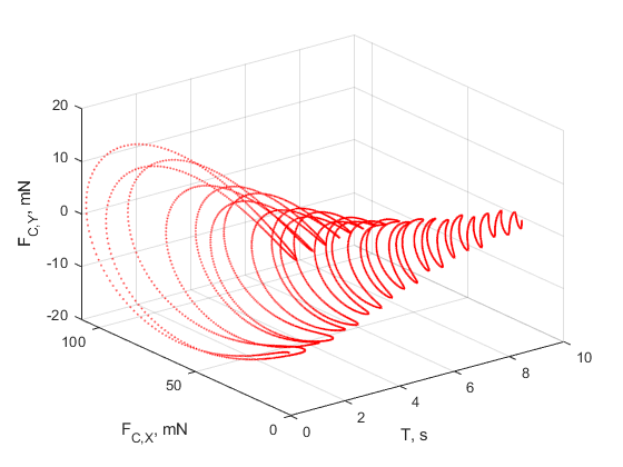
This figure shows the constraint forces that act on the weld joint. The longitudinal constraint force aligns with the x-axes of the weld joint frames. The transverse constraint force aligns with the y-axes. The constraint force along the z-axes is negligible because the motion of the double-pendulum model remains in the xy-plane.

You can use the Weld Joint block to measure the constraint force that the follower frame exerts on the base frame or, alternatively, the constraint force that the base frame exerts on the follower frame. The forces have the same magnitude but opposite directions. In this example, the Weld Joint block measures the constraint force that the follower frame exerts on the base frame.
You can also specify the frame to resolve the measured constraint forces. The resolution frame can be either the base or follower frame. Certain joint blocks, such as the 6-DOF Joint block, can have different orientations for the base and follower frames, which causes the same measurement to differ depending on the choice of the resolution frame.
Add Weld Joint Block to Model
To open the double-pendulum model, at the MATLAB® command prompt, enter
openExample("sm/DocDoublePendulumModelExample").Click the arrow in the bottom-left corner of the
Binary
                                    Link A1
subsystem to view the subsystem contents.Add a Weld Joint block and connect the blocks as shown in the figure.

Measure and Output Constraint Force
In the Weld Joint block dialog box, select Constraint Force. The block exposes a physical signal output port labeled fc.
Add a Connection Port block to the subsystem, name the block
Conn3, and connect the blocks as shown in the figure. Return to the top-level model.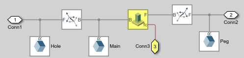
Add these blocks to the model.
Library Block Simscape > Utilities PS-Simulink Converter Simulink > Sinks To Workspace Connect the blocks as shown in the figure.

Specify these block parameters.
Block Dialog Box Parameter Value PS-Simulink Converter Vector format 1-D arrayOutput signal unit mNTo Workspace Variable name fcf_weld
Specify Damping
For each Revolute Joint block, in the
dialog box, set Internal Mechanics > Damping Coefficient to 1e-5 N*m/(deg/s). The damping coefficient
enables you to model energy dissipation during motion, so that the
double-pendulum model eventually comes to rest.
Simulate Model
In the Modeling tab, click Model Settings.
In the left pane of the Configuration Parameters window, click Solver, and set Solver to
ode15s(stiff/NDF). This solver is recommended for physical models.Expand Solver details and set the Max step size parameter to
0.001s.Run the simulation. Multibody Explorer opens with a dynamic view of the model. In the Views section, click the Isometric View button to view the double pendulum from an isometric perspective.

Plot Constraint Forces
At the MATLAB command prompt, enter the following plot commands:
figure;
plot3(fcf_weld.time, fcf_weld.data(:,1), fcf_weld.data(:,2),...
'.', 'MarkerSize', 1, 'Color', 'r');
grid on;
xlabel('T, s');
ylabel('F_{C,X}, mN');
zlabel('F_{C,Y}, mN');