Tuning of a Two-Loop Autopilot
This example shows how to use Simulink® Control Design™ to tune a two-loop autopilot controlling the pitch rate and vertical acceleration of an airframe.
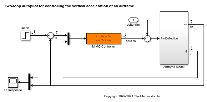
Model of Airframe Autopilot
The airframe dynamics and the autopilot are modeled in Simulink.
open_system('rct_airframe1')
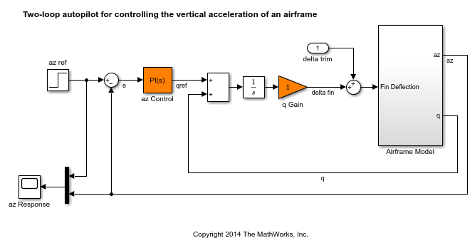
The autopilot consists of two cascaded loops. The inner loop controls the pitch rate q, and the outer loop controls the vertical acceleration az in response to the pilot stick command azref. In this architecture, the tunable elements include the PI controller gains ("az Control" block) and the pitch-rate gain ("q Gain" block). The autopilot must be tuned to respond to a step command azref in about 1 second with minimal overshoot. In this example, we tune the autopilot gains for one flight condition corresponding to zero incidence and a speed of 984 m/s.
To analyze the airframe dynamics, trim the airframe for  and
and  . The trim condition corresponds to zero normal acceleration and pitching moment (
 and
and  steady). Use
 findop to compute the corresponding closed-loop operating condition. Note that we added a "delta trim" input port so that findop can adjust the fin deflection to produce the desired equilibrium of forces and moments.
opspec = operspec('rct_airframe1');

% Specify trim condition
% Xe,Ze: known, not steady
opspec.States(1).Known = [1;1];
opspec.States(1).SteadyState = [0;0];
% u,w: known, w steady
opspec.States(3).Known = [1 1];
opspec.States(3).SteadyState = [0 1];
% theta: known, not steady
opspec.States(2).Known = 1;
opspec.States(2).SteadyState = 0;
% q: unknown, steady
opspec.States(4).Known = 0;
opspec.States(4).SteadyState = 1;
% integrator states unknown, not steady
opspec.States(5).SteadyState = 0;
opspec.States(6).SteadyState = 0;

op = findop('rct_airframe1',opspec);
 Operating point search report:
---------------------------------

opreport =


 Operating point search report for the Model rct_airframe1.
 (Time-Varying Components Evaluated at time t=0)

Operating point search completed successfully using optimization.
States:
----------
    Min          x          Max        dxMin        dx         dxMax
___________ ___________ ___________ ___________ ___________ ___________

(1.) rct_airframe1/Airframe Model/Aerodynamics & Equations of Motion/ Equations of Motion (Body Axes)/Position
     0           0           0         -Inf         984         Inf
-3047.9999  -3047.9999  -3047.9999     -Inf          0          Inf
(2.) rct_airframe1/Airframe Model/Aerodynamics & Equations of Motion/ Equations of Motion (Body Axes)/Theta
     0           0           0         -Inf     -0.0097235      Inf
(3.) rct_airframe1/Airframe Model/Aerodynamics & Equations of Motion/ Equations of Motion (Body Axes)/U,w
    984         984         984        -Inf       22.6897       Inf
     0           0           0           0      -1.4367e-11      0
(4.) rct_airframe1/Airframe Model/Aerodynamics & Equations of Motion/ Equations of Motion (Body Axes)/q
   -Inf     -0.0097235      Inf          0      1.7215e-16       0
(5.) rct_airframe1/Integrator
   -Inf     0.00070807      Inf        -Inf     -0.0097235      Inf
(6.) rct_airframe1/az Control/Integrator/Continuous/Integrator
   -Inf          0          Inf        -Inf     0.00024207      Inf

Inputs:
----------
   Min         u         Max
__________ __________ __________

(1.) rct_airframe1/delta trim
   -Inf    0.00070807    Inf

Outputs: None
----------
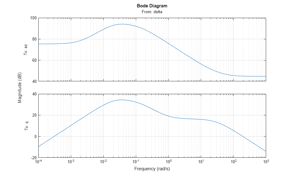
Linearize the "Airframe Model" block for the computed trim condition op and plot the gains from the fin deflection delta to az and q:
G = linearize('rct_airframe1','rct_airframe1/Airframe Model',op);
G.InputName = 'delta';
G.OutputName = {'az','q'};

bodemag(G), grid
Note that the airframe model has an unstable pole:
pole(G)
ans =

   -0.0320
   -0.0255
    0.1253
  -29.4685
Frequency-Domain Tuning with LOOPTUNE
You can use the looptune function to automatically tune multi-loop control systems subject to basic requirements such as integral action, adequate stability margins, and desired bandwidth. To apply looptune to the autopilot model, create an instance of the slTuner interface and designate the Simulink blocks "az Control" and "q Gain" as tunable. Also specify the trim condition op to correctly linearize the airframe dynamics.
ST0 = slTuner('rct_airframe1',{'az Control','q Gain'},op);
Mark the reference, control, and measurement signals as points of interest for analysis and tuning.
addPoint(ST0,{'az ref','delta fin','az','q'});
Finally, tune the control system parameters to meet the 1 second response time requirement. In the frequency domain, this roughly corresponds to a gain crossover frequency wc = 5 rad/s for the open-loop response at the plant input "delta fin".
wc = 5;
Controls = 'delta fin';
Measurements = {'az','q'};
[ST,gam,Info] = looptune(ST0,Controls,Measurements,wc);
Final: Peak gain = 1.01, Iterations = 71
The requirements are normalized so a final value near 1 means that all requirements are met. Confirm this by graphically validating the design.
figure('Position',[100,100,560,714])
loopview(ST,Info)
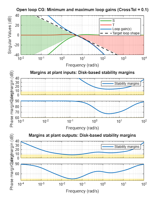
The first plot confirms that the open-loop response has integral action and the desired gain crossover frequency while the second plot shows that the MIMO stability margins are satisfactory (the blue curve should remain below the yellow bound). Next check the response from the step command azref to the vertical acceleration az:
T = getIOTransfer(ST,'az ref','az');
figure
step(T,5)
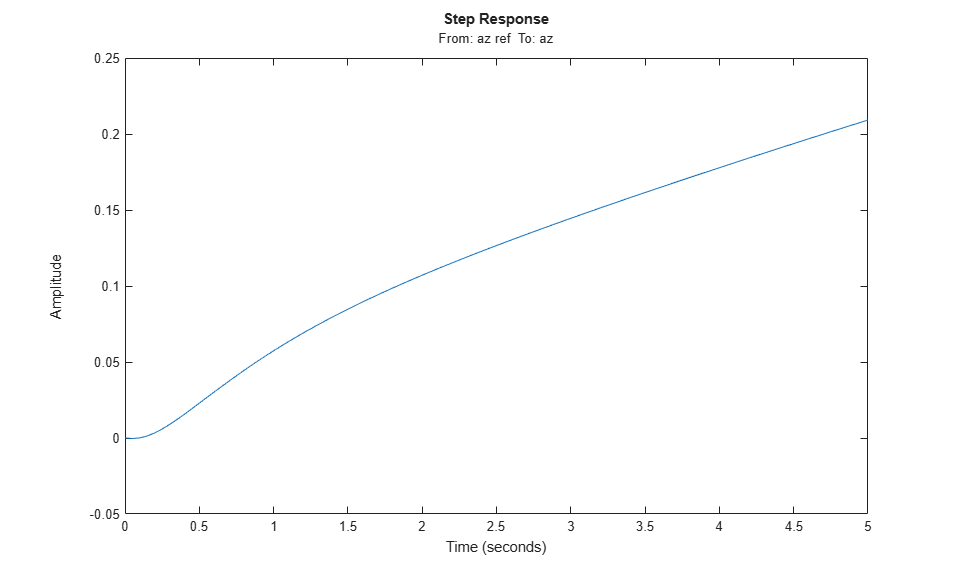
The acceleration az does not track azref despite the presence of an integrator in the loop. This is because the feedback loop acts on the two variables az and q and we have not specified which one should track azref.
Adding a Tracking Requirement
To remedy this issue, add an explicit requirement that az should follow the step command azref with a 1 second response time. Also relax the gain crossover requirement to the interval [3,12] to let the tuner find the appropriate gain crossover frequency.
TrackReq = TuningGoal.Tracking('az ref','az',1);
ST = looptune(ST0,Controls,Measurements,[3,12],TrackReq);
Final: Peak gain = 1.23, Iterations = 54
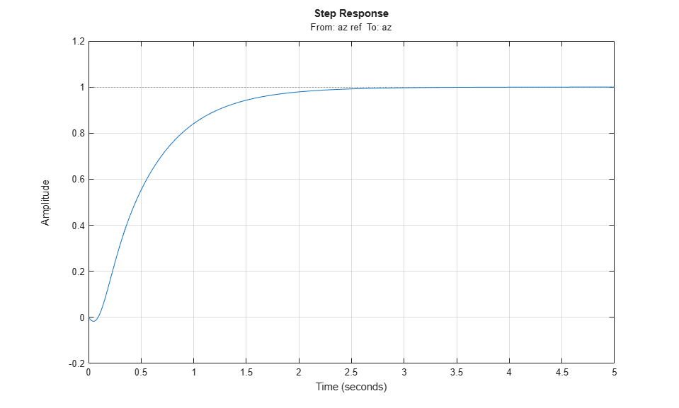
The step response from azref to az is now satisfactory:
Tr1 = getIOTransfer(ST,'az ref','az');
step(Tr1,5)
grid
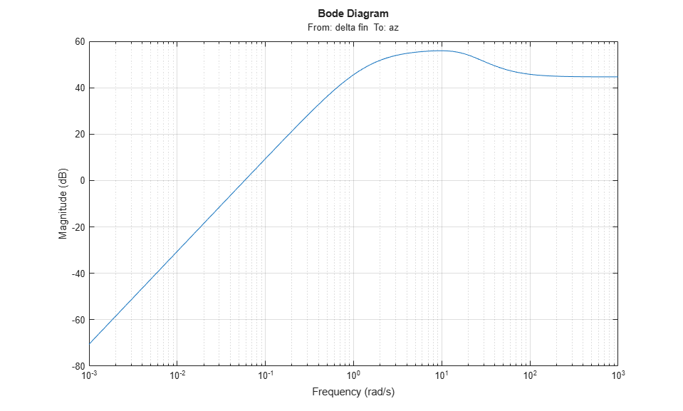
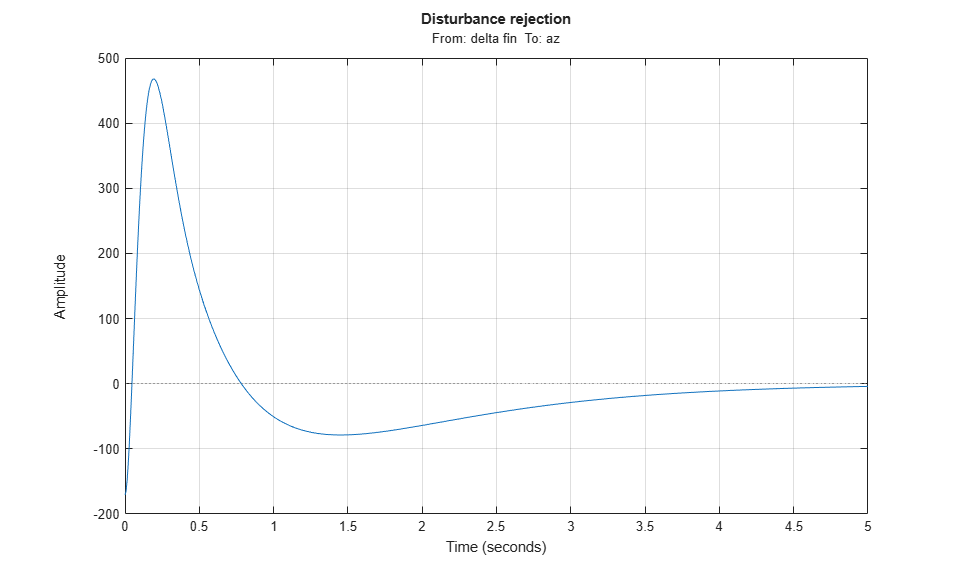
Also check the disturbance rejection characteristics by looking at the responses from a disturbance entering at the plant input.
Td1 = getIOTransfer(ST,'delta fin','az');
bodemag(Td1)
grid
step(Td1,5)
grid
title('Disturbance rejection')
Use showBlockValue to see the tuned values of the PI controller and inner-loop gain.
showBlockValue(ST)
AnalysisPoints_ =

  D =
       u1  u2  u3  u4
   y1   1   0   0   0
   y2   0   1   0   0
   y3   0   0   1   0
   y4   0   0   0   1

Name: AnalysisPoints_
Static gain.
-----------------------------------
az_Control =

             1
  Kp + Ki * ---
             s

  with Kp = 0.00166, Ki = 0.0017

Name: az_Control
Continuous-time PI controller in parallel form.
-----------------------------------
q_Gain =

  D =
          u1
   y1  1.985

Name: q_Gain
Static gain.
If this design is satisfactory, use writeBlockValue to apply the tuned values to the Simulink model and simulate the tuned controller in Simulink.
writeBlockValue(ST)
MIMO Design with SYSTUNE
Cascaded loops are commonly used for autopilots. Yet one may wonder how a single MIMO controller that uses both az and q to generate the actuator command delta fin would compare with the two-loop architecture. Trying new control architectures is easy with systune or looptune. For variety, we now use systune to tune the following MIMO architecture.
open_system('rct_airframe2')
As before, compute the trim condition for and .
opspec = operspec('rct_airframe2');

% Specify trim condition
% Xe,Ze: known, not steady
opspec.States(1).Known = [1;1];
opspec.States(1).SteadyState = [0;0];
% u,w: known, w steady
opspec.States(3).Known = [1 1];
opspec.States(3).SteadyState = [0 1];
% theta: known, not steady
opspec.States(2).Known = 1;
opspec.States(2).SteadyState = 0;
% q: unknown, steady
opspec.States(4).Known = 0;
opspec.States(4).SteadyState = 1;
% controller states unknown, not steady
opspec.States(5).SteadyState = [0;0];

op = findop('rct_airframe2',opspec);
 Operating point search report:
---------------------------------

opreport =


 Operating point search report for the Model rct_airframe2.
 (Time-Varying Components Evaluated at time t=0)

Operating point search completed successfully using optimization.
States:
----------
    Min          x          Max        dxMin        dx         dxMax
___________ ___________ ___________ ___________ ___________ ___________

(1.) rct_airframe2/Airframe Model/Aerodynamics & Equations of Motion/ Equations of Motion (Body Axes)/Position
     0           0           0         -Inf         984         Inf
-3047.9999  -3047.9999  -3047.9999     -Inf          0          Inf
(2.) rct_airframe2/Airframe Model/Aerodynamics & Equations of Motion/ Equations of Motion (Body Axes)/Theta
     0           0           0         -Inf     -0.0097235      Inf
(3.) rct_airframe2/Airframe Model/Aerodynamics & Equations of Motion/ Equations of Motion (Body Axes)/U,w
    984         984         984        -Inf       22.6897       Inf
     0           0           0           0      2.4588e-11       0
(4.) rct_airframe2/Airframe Model/Aerodynamics & Equations of Motion/ Equations of Motion (Body Axes)/q
   -Inf     -0.0097235      Inf          0      -4.0169e-16      0
(5.) rct_airframe2/MIMO Controller
   -Inf     0.00065361      Inf        -Inf     -0.0089973      Inf
   -Inf     1.0577e-18      Inf        -Inf      0.030259       Inf

Inputs:
----------
   Min         u         Max
__________ __________ __________

(1.) rct_airframe2/delta trim
   -Inf    0.00043574    Inf

Outputs: None
----------
As with looptune, use the slTuner interface to configure the Simulink model for tuning. Note that the signals of interest are already marked as Linear Analysis points in the Simulink model.
ST0 = slTuner('rct_airframe2','MIMO Controller',op);
Try a second-order MIMO controller with zero feedthrough from e to delta fin. To do this, create the desired controller parameterization and associate it with the "MIMO Controller" block using setBlockParam:
C0 = tunableSS('C',2,1,2);         % Second-order controller
C0.D.Value(1) = 0;                 % Fix D(1) to zero
C0.D.Free(1) = false;
setBlockParam(ST0,'MIMO Controller',C0)
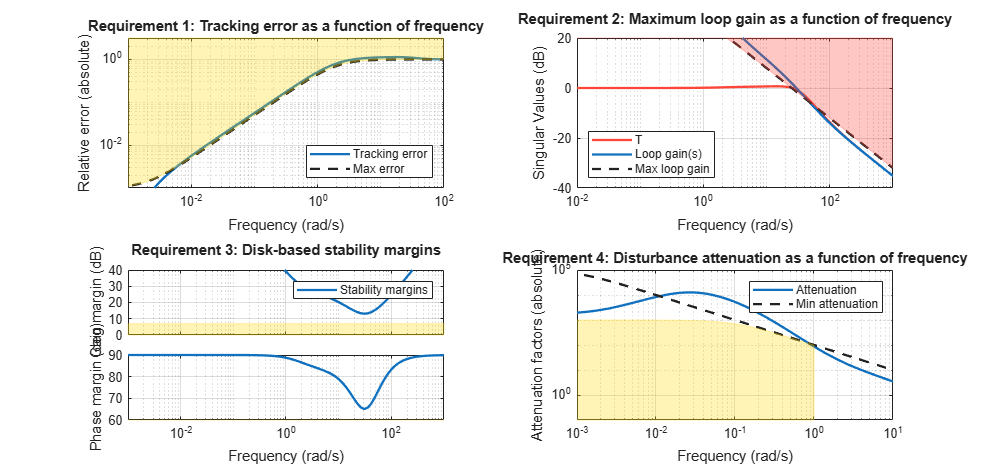
Next create the tuning requirements. Here we use the following four requirements:
Tracking:
azshould respond in about 1 second to theazrefcommandBandwidth and roll-off: The loop gain at
delta finshould roll off after 25 rad/s with a -20 dB/decade slopeStability margins: The margins at
delta finshould exceed 7 dB and 45 degreesDisturbance rejection: The attenuation factor for input disturbances should be 40 dB at 1 rad/s increasing to 100 dB at 0.001 rad/s.
% Tracking
Req1 = TuningGoal.Tracking('az ref','az',1);

% Bandwidth and roll-off
Req2 = TuningGoal.MaxLoopGain('delta fin',tf(25,[1 0]));

% Margins
Req3 = TuningGoal.Margins('delta fin',7,45);

% Disturbance rejection
% Use an FRD model to sketch the desired attenuation profile with a few points
Freqs = [0 0.001 1];
MinAtt = [100 100 40];  % in dB
Req4 = TuningGoal.Rejection('delta fin',frd(db2mag(MinAtt),Freqs));
Req4.Focus = [0 1];
You can now use systune to tune the controller parameters subject to these requirements.
AllReqs = [Req1,Req2,Req3 Req4];
Opt = systuneOptions('RandomStart',3);

rng(0)
[ST,fSoft] = systune(ST0,AllReqs,Opt);
Final: Soft = 1.42, Hard = -Inf, Iterations = 47
Final: Soft = 1.42, Hard = -Inf, Iterations = 62
Final: Soft = 1.14, Hard = -Inf, Iterations = 81
Final: Soft = 1.14, Hard = -Inf, Iterations = 128
The best design has an overall objective value close to 1, indicating that all four requirements are nearly met. Use viewGoal to inspect each requirement for the best design.
figure('Position',[100,100,987,474])
viewGoal(AllReqs,ST)
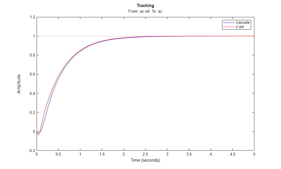
Compute the closed-loop responses and compare with the two-loop design.
T = getIOTransfer(ST,{'az ref','delta fin'},'az');

figure
step(Tr1,'b',T(1),'r',5)
title('Tracking')
legend('Cascade','2 dof')
step(Td1,'b',T(2),'r',5)
title('Disturbance rejection')
legend('Cascade','2 dof')
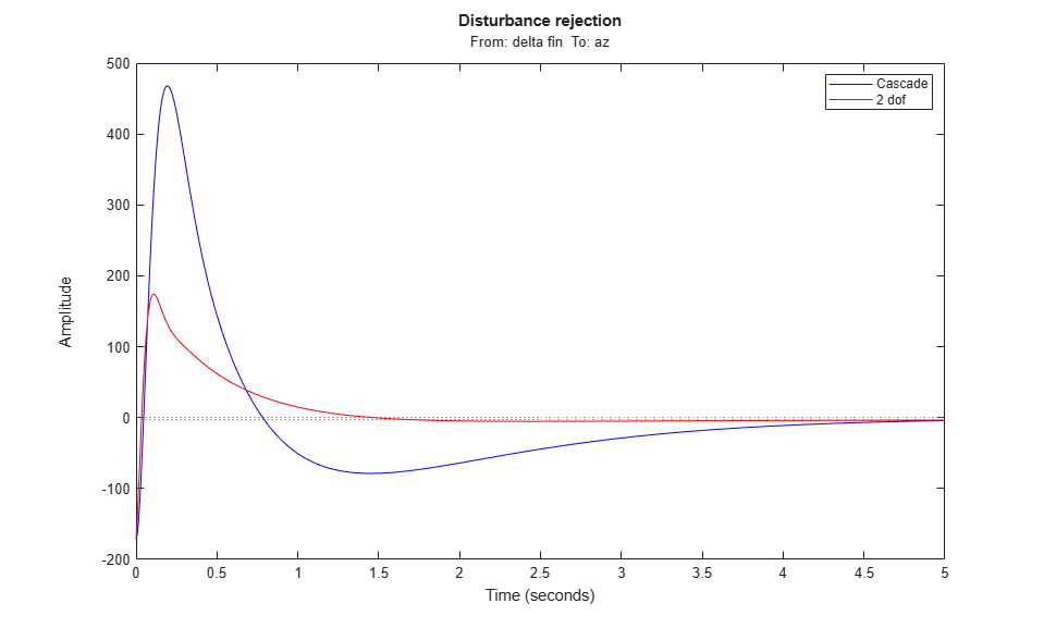
The tracking performance is similar but the second design has better disturbance rejection properties.