Tuning of a Digital Motion Control System
This example shows how to use Control System Toolbox™ to tune a digital motion control system.
Motion Control System
The motion system under consideration is shown below.
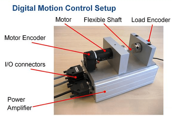
Figure 1: Digital motion control hardware
This device could be part of some production machine and is intended to move some load (a gripper, a tool, a nozzle, or anything else that you can imagine) from one angular position to another and back again. This task is part of the "production cycle" that has to be completed to create each product or batch of products.
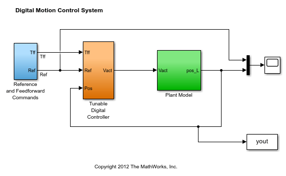
The digital controller must be tuned to maximize the production speed of the machine without compromising accuracy and product quality. To do this, we first model the control system in Simulink® using a 4th-order model of the inertia and flexible shaft:
open_system('rct_dmc')
The "Tunable Digital Controller" consists of a gain in series with a lead/lag controller.
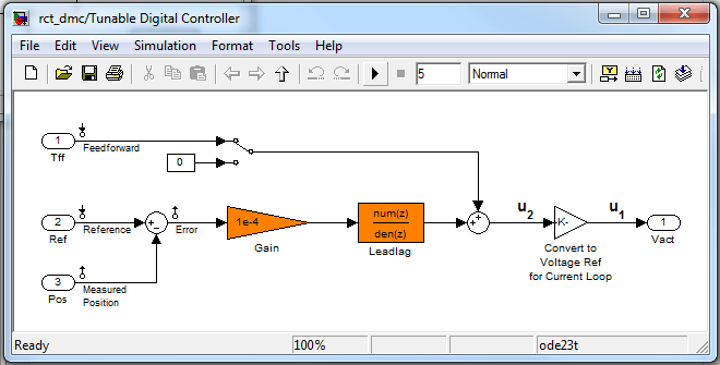
Figure 2: Digital controller
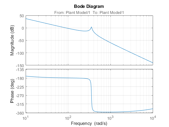
Tuning is complicated by the presence of a flexible mode near 350 rad/s in the plant:
G = linearize('rct_dmc','rct_dmc/Plant Model');
bode(G,{10,1e4}), grid
Compensator Tuning
We are seeking a 0.5 second response time to a step command in angular position with minimum overshoot. This corresponds to a target bandwidth of approximately 5 rad/s. The looptune command offers a convenient way to tune fixed-structure compensators like the one in this application. To use looptune, first instantiate the slTuner interface to automatically acquire the control structure from Simulink. Note that the signals of interest are already marked as Linear Analysis Points in the Simulink model.
ST0 = slTuner('rct_dmc',{'Gain','Leadlag'});
Next use looptune to tune the compensator parameters for the target gain crossover frequency of 5 rad/s:
Measurement = 'Measured Position';  % controller input
Control = 'Leadlag';                % controller output
ST1 = looptune(ST0,Control,Measurement,5);
Final: Peak gain = 0.979, Iterations = 19
Achieved target gain value TargetGain=1.
A final value below or near 1 indicates success. Inspect the tuned values of the gain and lead/lag filter:
showTunable(ST1)
Block 1: rct_dmc/Tunable Digital Controller/Gain =

  D =
              u1
   y1  1.869e-05

Name: Gain
Static gain.

-----------------------------------

Block 2: rct_dmc/Tunable Digital Controller/Leadlag =

  3.856 s + 6.323
  ---------------
     s + 13.35

Name: Leadlag
Continuous-time transfer function.
Design Validation
To validate the design, use the slTuner interface to quickly access the closed-loop transfer functions of interest and compare the responses before and after tuning.
T0 = getIOTransfer(ST0,'Reference','Measured Position');
T1 = getIOTransfer(ST1,'Reference','Measured Position');
step(T0,T1), grid
legend('Original','Tuned')
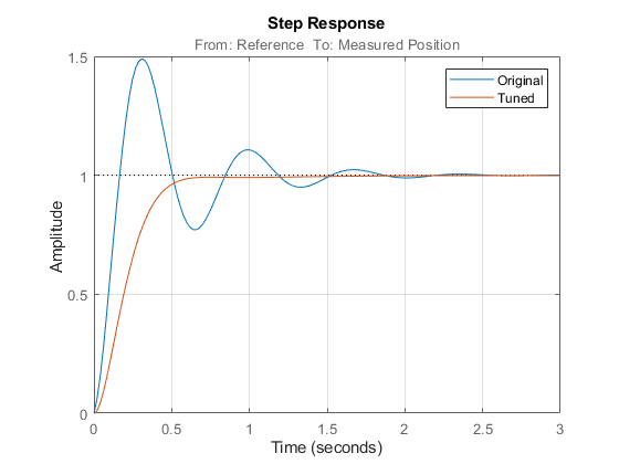
The tuned response has significantly less overshoot and satisfies the response time requirement. However these simulations are obtained using a continuous-time lead/lag compensator (looptune operates in continuous time) so we need to further validate the design in Simulink using a digital implementation of the lead/lag compensator. Use writeBlockValue to apply the tuned values to the Simulink model and automatically discretize the lead/lag compensator to the rate specified in Simulink.
writeBlockValue(ST1)
You can now simulate the response of the continuous-time plant with the digital controller:
sim('rct_dmc');  % angular position logged in "yout" variable
t = yout.time;
y = yout.signals.values;
step(T1), hold, plot(t,y,'r--')
legend('Continuous','Hybrid (Simulink)')
Current plot held
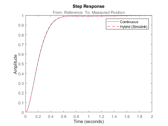
The simulations closely match and the coefficients of the digital lead/lag can be read from the "Leadlag" block in Simulink.
Tuning an Additional Notch Filter
Next try to increase the control bandwidth from 5 to 50 rad/s. Because of the plant resonance near 350 rad/s, the lead/lag compensator is no longer sufficient to get adequate stability margins and small overshoot. One remedy is to add a notch filter as shown in Figure 3.
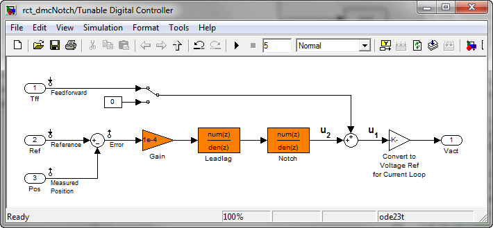
Figure 3: Digital Controller with Notch Filter
To tune this modified control architecture, create an slTuner instance with the three tunable blocks.
ST0 = slTuner('rct_dmcNotch',{'Gain','Leadlag','Notch'});
By default the "Notch" block is parameterized as any second-order transfer function. To retain the notch structure
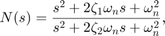
specify the coefficients  as real parameters and create a parametric model
 N of the transfer function shown above:
wn = realp('wn',300);
zeta1 = realp('zeta1',1);
zeta2 = realp('zeta2',1);
zeta1.Minimum = 0;   zeta1.Maximum = 1;   % 0 <= zeta1 <= 1
zeta2.Minimum = 0;   zeta2.Maximum = 1;   % 0 <= zeta2 <= 1
N = tf([1 2*zeta1*wn wn^2],[1 2*zeta2*wn wn^2]);  % tunable notch filter
Then associate this parametric notch model with the "Notch" block in the Simulink model. Because the control system is tuned in the continuous time, you can use a continuous-time parameterization of the notch filter even though the "Notch" block itself is discrete.
setBlockParam(ST0,'Notch',N);
Next use looptune to jointly tune the "Gain", "Leadlag", and "Notch" blocks with a 50 rad/s target crossover frequency. To eliminate residual oscillations from the plant resonance, specify a target loop shape with a -40 dB/decade roll-off past 50 rad/s.
% Specify target loop shape with a few frequency points
Freqs = [5 50 500];
Gains = [10 1 0.01];
TLS = TuningGoal.LoopShape('Notch',frd(Gains,Freqs));

Measurement = 'Measured Position';  % controller input
Control = 'Notch';                  % controller output
ST2 = looptune(ST0,Control,Measurement,TLS);
Final: Peak gain = 1.05, Iterations = 60
The final gain is close to 1, indicating that all requirements are met. Compare the closed-loop step response with the previous designs.
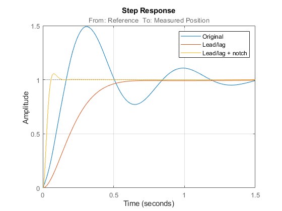
T2 = getIOTransfer(ST2,'Reference','Measured Position');
clf
step(T0,T1,T2,1.5), grid
legend('Original','Lead/lag','Lead/lag + notch')

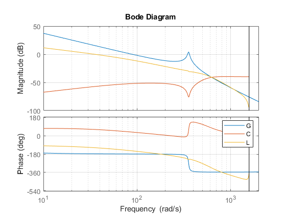
To verify that the notch filter performs as expected, evaluate the total compensator C and the open-loop response L and compare the Bode responses of G, C, L:
% Get tuned block values (in the order blocks are listed in ST2.TunedBlocks)
[g,LL,N] = getBlockValue(ST2,'Gain','Leadlag','Notch');
C = N * LL * g;

L = getLoopTransfer(ST2,'Notch',-1);

bode(G,C,L,{1e1,1e3}), grid
legend('G','C','L')
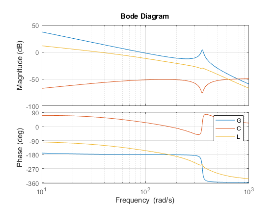
This Bode plot confirms that the plant resonance has been correctly "notched out."
Discretizing the Notch Filter
Again use writeBlockValue to discretize the tuned lead/lag and notch filters and write their values back to Simulink. Compare the MATLAB® and Simulink responses:
writeBlockValue(ST2)

sim('rct_dmcNotch');
t = yout.time;
y = yout.signals.values;
step(T2), hold, plot(t,y,'r--')
legend('Continuous','Hybrid (Simulink)')
Current plot held
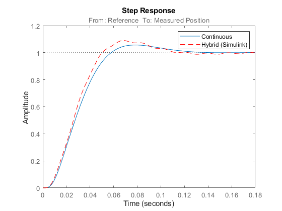
The Simulink response exhibits small residual oscillations. The notch filter discretization is the likely culprit because the notch frequency is close to the Nyquist frequency pi/0.002=1570 rad/s. By default the notch is discretized using the ZOH method. Compare this with the Tustin method prewarped at the notch frequency:
wn = damp(N);  % natural frequency of the notch filter
Ts = 0.002;    % sample time of discrete notch filter

Nd1 = c2d(N,Ts,'zoh');
Nd2 = c2d(N,Ts,'tustin',c2dOptions('PrewarpFrequency',wn(1)));

clf, bode(N,Nd1,Nd2)
legend('Continuous','Discretized with ZOH','Discretized with Tustin',...
    'Location','NorthWest')
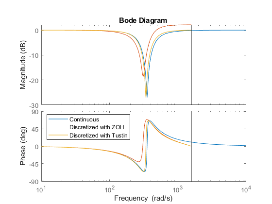
The ZOH method has significant distortion and prewarped Tustin should be used instead. To do this, specify the desired rate conversion method for the notch filter block:
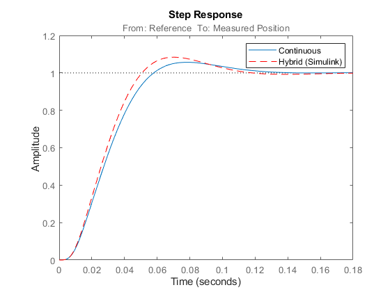
setBlockRateConversion(ST2,'Notch','tustin',wn(1))

writeBlockValue(ST2)
writeBlockValue now uses Tustin prewarped at the notch frequency to discretize the notch filter and write it back to Simulink. Verify that this gets rid of the oscillations.
sim('rct_dmcNotch');
t = yout.time;
y = yout.signals.values;
step(T2), hold, plot(t,y,'r--')
legend('Continuous','Hybrid (Simulink)')
Current plot held
Direct Discrete-Time Tuning
Alternatively, you can tune the controller directly in discrete time to avoid discretization issues with the notch filter. To do this, specify that the Simulink model should be linearized and tuned at the controller sample time of 0.002 seconds:
ST0 = slTuner('rct_dmcNotch',{'Gain','Leadlag','Notch'});
ST0.Ts = 0.002;
To prevent high-gain control and saturations, add a requirement that limits the gain from reference to control signal (output of Notch block).
GL = TuningGoal.Gain('Reference','Notch',0.01);
Now retune the controller at the specified sampling rate and verify the tuned open- and closed-loop responses.
ST2 = looptune(ST0,Control,Measurement,TLS,GL);

% Closed-loop responses
T2 = getIOTransfer(ST2,'Reference','Measured Position');
clf
step(T0,T1,T2,1.5), grid
legend('Original','Lead/lag','Lead/lag + notch')
Final: Peak gain = 1.04, Iterations = 39
% Open-loop responses
[g,LL,N] = getBlockValue(ST2,'Gain','Leadlag','Notch');
C = N * LL * g;
L = getLoopTransfer(ST2,'Notch',-1);
bode(G,C,L,{1e1,2e3}), grid
legend('G','C','L')
The results are similar to those obtained when tuning the controller in continuous time. Now validate the digital controller against the continuous-time plant in Simulink.
writeBlockValue(ST2)

sim('rct_dmcNotch');
t = yout.time;
y = yout.signals.values;
step(T2), hold, plot(t,y,'r--')
legend('Discrete','Hybrid (Simulink)')
Current plot held
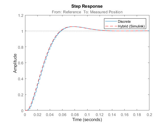
This time, the hybrid response closely matches its discrete-time approximation and no further adjustment of the notch filter is required.