Design Compensator Using Automated PID Tuning and Graphical Bode Design

R2026b

This example shows how to design a compensator for a Simulink^® model using automated PID tuning in the Control System Designer app. It then shows how to fine tune the compensator design using the open-loop Bode editor.

Water Tank Model

Open the watertank_comp_design model.

open_system("watertank_comp_design")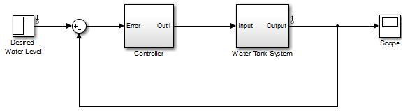

This model contains a water-tank plant model and a PID controller in a single-loop feedback configuration. To view the water tank model, open the Water-Tank System subsystem.

open_system("watertank_comp_design/Water-Tank System")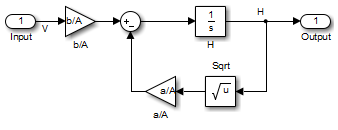

This model represents the following water tank system.

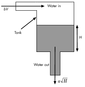
Here:

• $H$ is the height of water in the tank.

• $\text{Vol}$ is the volume of water in the tank.

• $V$ is the voltage applied to the pump.

• $A$ is the cross-sectional area of the tank.

• $b$ is a constant related to the flow rate into the tank.

• $a$ is a constant related to the flow rate out of the tank.

Water enters the tank from the top at a rate proportional to the voltage applied to the pump. The water leaves through an opening in the tank base at a rate that is proportional to the square root of the water height in the tank. The presence of the square root in the water flow rate results in a nonlinear plant. Based on these flow rates, the rate of change of the tank volume is:

$$\frac{d}{dt}Vol=A\frac{dH}{dt}=bV-a\sqrt{H}$$

Design Requirements

Tune the PID controller to meet the following closed-loop step response design requirements:

• Overshoot less than 5%

• Rise time less than five seconds

Open Control System Designer

To open Control System Designer, in the Simulink model window, in the Apps gallery, click Control System Designer.

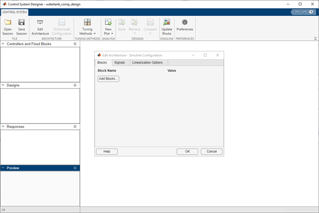
Control System Designer opens and automatically opens the Edit Architecture dialog box.

Specify Blocks to Tune

To specify the compensator to tune, in the Edit Architecture dialog box, click Add Blocks.

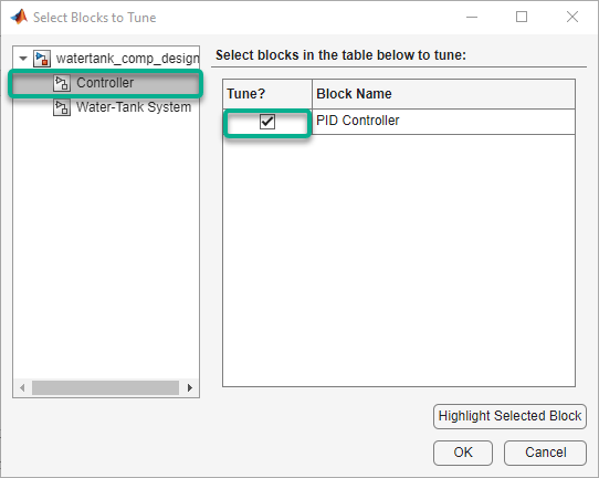
In the Select Blocks to Tune dialog box, in the left pane, click the Controller subsystem. In the Tune column, check the box for the PID Controller.

Click OK.

In the Edit Architecture dialog box, the app adds the selected controller block to the list of blocks to tune on the Blocks tab. On the Signals tab, the app also adds the output of the PID Controller block to the list of analysis point Locations.

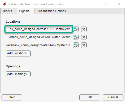
When Control System Designer opens, it adds any analysis points previously defined in the Simulink model to the Locations list. For the watertank_comp_design, there are two such signals.

• Desired Water Level block output — Reference signal for the closed-loop step response

• Water-Tank System block output — Output signal for the closed-loop step response

To linearize the Simulink model and set the control architecture, click OK.

By default, Control System Designer linearizes the plant model at the model initial conditions.

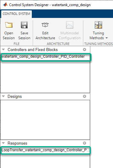
The app adds the PID controller to the data browser, in the Controllers and Fixed Blocks section. The app also computes the open-loop transfer function at the output of the PID Controller block and adds this response to the data browser.

Plot Closed-Loop Step Response

To analyze the controller design, create a closed-loop transfer function of the system and plot its step response.

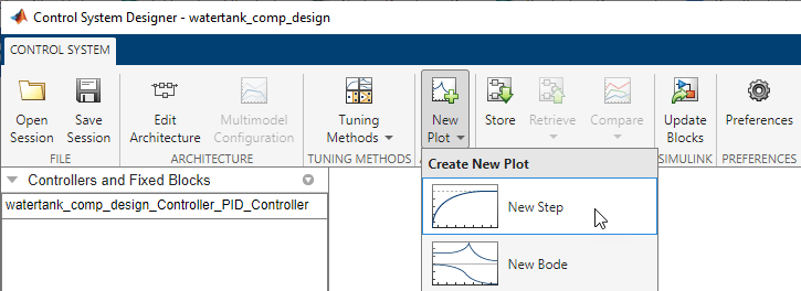
On the Control System tab, click New Plot, and select New Step.

In the New Step dialog box, in the Select Response to Plot drop-down list, select New Input-Output Transfer Response.

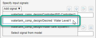
To add an input signal, under Specify input signals, in the Add signal drop-down list, select the output of the Desired Water Level block.

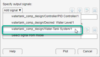
To add an output signal, under Specify output signals, in the Add signal drop-down list, select the output of the Water-Tank System block.

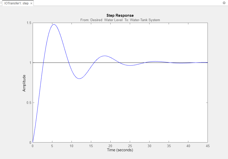
To create the closed-loop transfer function and plot the step response, click Plot.

To view the maximum overshoot on the response plot, right-click the plot area, and select Characteristics > Peak Response.

To view the rise time on the response plot, right-click the plot area, and select Characteristics > Rise Time.

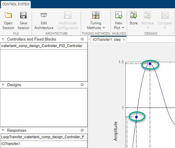
Mouse-over the characteristic indicators to view their values. The current design has a:

• Maximum overshoot of 47.9%.

• Rise time of 2.13 seconds.

This response does not satisfy the 5% overshoot design requirement.

Tune Compensator Using Automated PID Tuning

To tune the compensator using automated PID tuning, click Tuning Methods, and select PID Tuning.

In the PID Tuning dialog box, in the Specifications section, select the following options:

• Tuning method — Robust response time

• Controller Type — PI

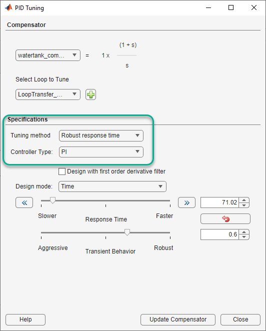
Click Update Compensator. The app updates the closed-loop response for the new compensator settings and updates the step response plot.

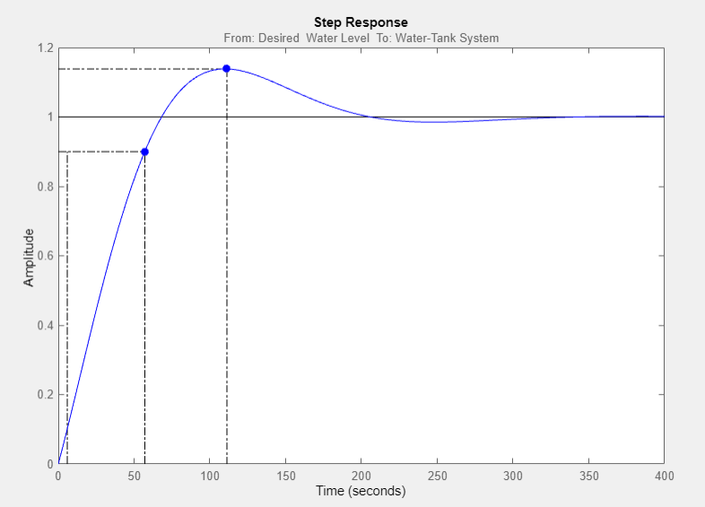
To check the system performance, mouse over the response characteristic markers. The system response with the tuned compensator has a:

• Maximum overshoot of 13.8%.

• Rise time of 51.2 seconds.

This response exceeds the maximum allowed overshoot of 5%. The rise time is much slower than the required rise time of five seconds.

Tune Compensator Using Bode Graphical Tuning

To decrease the rise time, interactively increase the compensator gain using graphical Bode Tuning.

To open the open-loop Bode editor, click Tuning Methods, and select Bode Editor.

In the Select response to edit dialog box, the open-loop response at the output of the PID Controller block is already selected. To open the Bode editor for this response, click Plot.

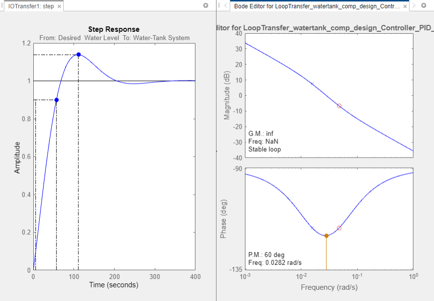
Tip

To view the Bode Editor and Step Response plots side-by-side, in the top-right corner of the document area, click the arrow and select Tile All > Left/Right.

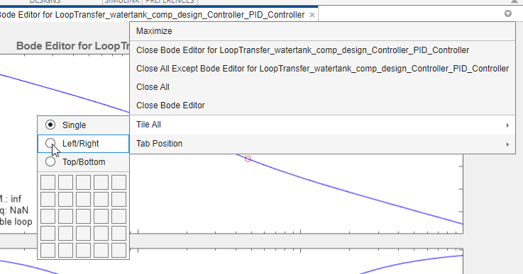
In the Bode Editor plot, drag the magnitude response up to increase the compensator gain. By increasing the gain, you increase the bandwidth and speed up the response.

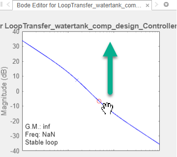
As you drag the Bode response upward, the app automatically updates the compensator and the associated response plots. Also, when you release the plot, the updated gain value displays on the right side of the app status bar.

Increase the compensator gain until the step response meets the design requirements. One potential solution is to set the gain to about 1.7.

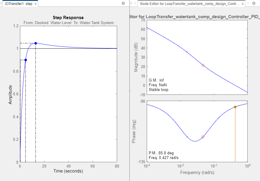
At this gain value, the closed loop response has a:

• Maximum overshoot of around 4.74%.

• Rise time of around 4.4 seconds.

Fine Tune Controller Using Compensator Editor

To tune the parameters of your compensator directly, use the Compensator Editor. In the Bode Editor, right-click the plot area, and select Edit Compensator.

In the Compensator Editor dialog box, on the Parameter tab, tune the PID controller gains. For more information on editing compensator parameters, see Tune Simulink Blocks Using Compensator Editor.

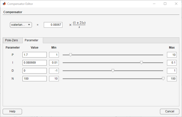
While the tuned compensator meets the design requirements, the settling time is over 30 seconds. To improve the settling time, adjust the P and I parameters of the controller manually.

For example, set the compensator parameters to:

• P = 4

• I = 0.1

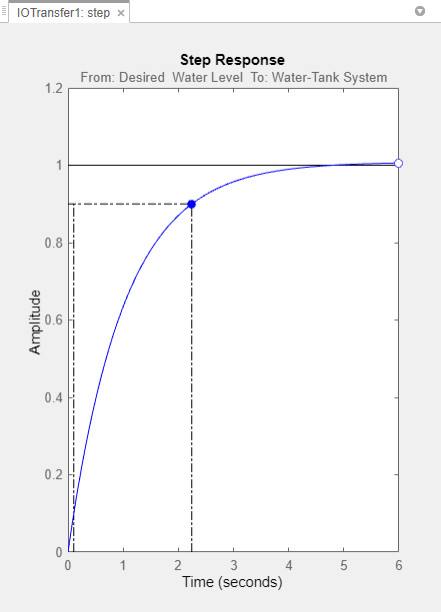
This compensator produces a closed-loop response with a:

• Maximum overshoot of 0.744%.

• Rise time of 2.14 seconds.

• Settling time of around three seconds.

Simulate Closed-Loop System in Simulink

Validate your compensator design by simulating the nonlinear Simulink model with the tuned controller parameters.

To write the tuned compensator parameters to the PID Controller block, in Control System Designer, on the Control System tab, click Update Blocks.

In the Simulink model window, run the simulation.

To view the closed-loop simulation output, open the Scope block.

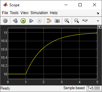
The closed-loop response of the nonlinear system satisfies the design requirements with a rise time of less than five seconds and minimal overshoot.