Design Active Disturbance Rejection Control for Boost Converter
This example shows how to design active disturbance rejection control (ADRC) for a DC-DC boost converter modeled in Simulink® using Simscape™ Electrical™ components. In this example, you also compare the ADRC control performance with a PID controller tuned on a linearized plant model.
Typically, you control power electronics systems using PID controllers whose gains are tuned using PID tuning tools with a linearized plant model. You can design PID controllers for linearized plant models in the following ways.
Estimate the plant frequency response over a range of frequencies. For an example, see Design Controller for Boost Converter Model Using Frequency Response Data.
Estimate the parameters of a linear model of the plant using System Identification Toolbox™ software. For an example, see Design Controller for Power Electronics Model Using Simulated I/O Data.
Although you can tune the PID controller over a wide operating range, designing experiments and tuning PID gains require significant efforts. Using ADRC you can obtain a nonlinear controller and achieve better performance with a simpler setup and less tuning effort.
Boost Converter Model
This example uses a DC-DC boost converter model that converts one DC voltage to another, typically higher, DC voltage by controlled chopping or switching of the source voltage.
mdl = 'scdBoostConverterADRC';
open_system(mdl)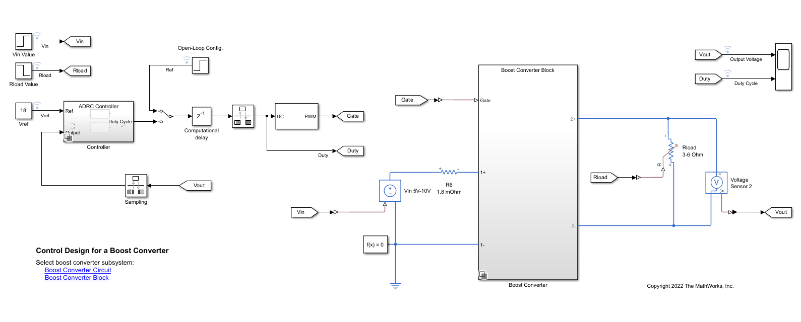
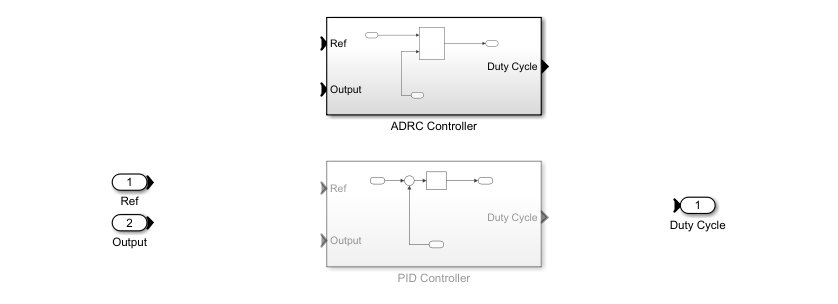
This model contains a controller variant subsystem with two choices: an ADRC controller and a PID controller. The ADRC Controller subsystem is set as the default active variant. The model also includes a manual switch to operate the model in open-loop and closed-loop configurations. It is set to an open-loop configuration by default.
The model uses a MOSFET driven by a pulse-width modulation (PWM) signal for switching. The controller adjusts the PWM duty cycle, , based on both the reference value and output voltage signals. The duty cycle regulates the output voltage to the reference value .
Simscape Electrical software contains predefined blocks for many power electronics systems. This model contains a variant subsystem with two versions of the boost converter model:
The
Boost Converter Circuitsubsystem is constructed using electrical power components. The parameters of the circuit components are based on [1].The
Boost Converter Blocksubsystem is constructed using the Boost Converter block and is configured to have the same parameters as the boost converter circuit. For more information on this block, see Boost Converter (Simscape Electrical). The model uses this subsystem by default.
Design ADRC Controller
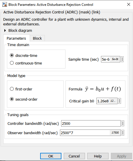
ADRC is a powerful tool for the controller design of a plant with unknown dynamics and internal and external disturbances. The block models unknown dynamics and disturbances as an extended state of the plant and estimates them using an observer. The block lets you design a controller using only a few key tuning parameters for the control algorithm:
Model order type (first-order or second order)
Critical gain of the model response
Controller and observer bandwidths
Additionally, you also specify the Time domain parameter to match the time domain of the plant model. In this example, it is set to discrete-time and with a sample time of 5e-6 seconds. The following sections describe how to find the remaining tuning parameters specified in the ADRC block parameters for this model.
Model Order and Critical Gain
To identify the model order, simulate the plant model in the open-loop configuration. Use a step input of 0.5 as duty cycle to drive the plant model.
set_param(mdl,'SignalLoggingName','openLoopSim');
sim(mdl);
figure;
Ref = getElement(openLoopSim,'Ref');
Vout = getElement(openLoopSim,'Output Voltage');
plot(Ref.Values.Time,Ref.Values.Data...
    ,Vout.Values.Time,Vout.Values.Data)
grid on
xlabel('Time (s)')
ylabel('Output Voltage (V)')
legend('Ref','Output')
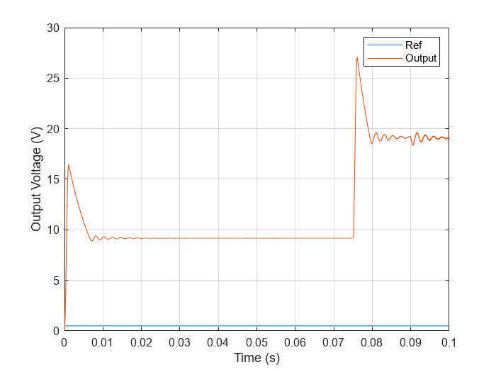
To determine the critical gain value b0, you can examine the output voltage response over a short interval of 0.0005 seconds right after the step reference input.
x = Vout.Values.Time(1:20091);
y = Vout.Values.Data(1:20091);
figure
plot(x,y)
xlabel('Time (s)')
ylabel('Output Voltage (V)')
grid on

Because this curve contains the effects of switching, use polyfit to get a better approximation of the output voltage over this time range.
[p,~,mu] = polyfit(x,y,3);
f = polyval(p,x,[],mu);
figure;
plot(x,y,x,f)
grid on
xlabel('Time (s)')
ylabel('Output Voltage (V)')
legend('Data','Polyfit','Location','best')

f(end)
ans =
7.9240
The output voltage shows a typical shape for a second-order dynamic system. As a result, select second-order for the Model type parameter. Based on the output voltage waveform, you can determine the critical gain through the second-order response approximation .
Over a duration of 0.0005 seconds, the output voltage changes by about 7.8594V.
Controller Bandwidth and Observer Bandwidth
The controller bandwidth usually depends on the performance specifications, either in the frequency domain or time domain. In this example, the controller bandwidth is 2500 rad/s. The observer needs to converge faster than the controller. In general, the observer bandwidth is set to 5 to 10 times . In this example, .
Toggle the manual switch to operate the model in the closed-loop configuration.
set_param('scdBoostConverterADRC/Manual Switch','sw','0')
Simulate the model.
set_param(mdl,'SignalLoggingName','adrcSim');
sim(mdl);
Vref = getElement(adrcSim,'Vref');
Vout_adrc = getElement(adrcSim,'Output Voltage');
figure;
plot(Vref.Values.Time,Vref.Values.Data...
    ,Vout_adrc.Values.Time,Vout_adrc.Values.Data)
grid on
xlim([0 0.03])
xlabel('Time (s)')
ylabel('Output Voltage (V)')
legend('Vref','Output')

Performance Comparison of ADRC and PID Controller
You can examine the tuned controller performance using a simulation with line and load disturbances. The model uses the following disturbances.
Line disturbance at t = 0.075 s, which increases the input voltage from 5 V to 10 V.
Load disturbance at t = 0.09 s, which increases the load resistance from 3 ohms to 6 ohms.
You compare the output voltage of the boost converter controlled using the ADRC controller with a PID controller tuned on a linear plant model obtained using frequency response estimation at the same operating point = 18 V.
Simulate the model with the PID Controller subsystem.
set_param([mdl,'/Controller'],'LabelModeActiveChoice','PID')
set_param(mdl,'SignalLoggingName','pidSim');
sim(mdl);
Vout_pid = getElement(pidSim,'Output Voltage');
Compare the performance of the two controllers.
figure;
plot(Vout_adrc.Values.Time,Vout_adrc.Values.Data...
    ,Vout_pid.Values.Time,Vout_pid.Values.Data)
grid on
xlabel('Time (s)')
ylabel('Output Voltage (V)')
legend('Vout (ADRC)','Vout (PID)')
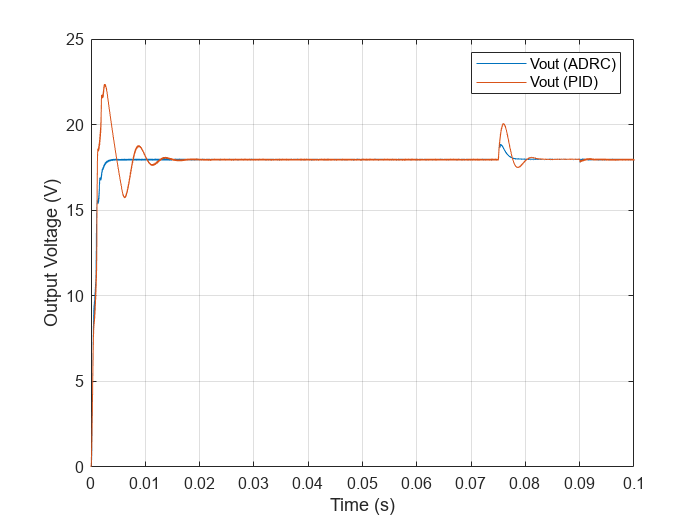
The ADRC controller drives the initial transient to the steady state much faster than the PID controller. You can further zoom in to take a closer look at how both controllers perform with the disturbances.
figure;
plot(Vout_adrc.Values.Time,Vout_adrc.Values.Data...
    ,Vout_pid.Values.Time,Vout_pid.Values.Data)
grid on
xlim([0.06 0.1])
xlabel('Time (s)')
ylabel('Output Voltage (V)')
legend('Vout (ADRC)','Vout (PID)')

After each disturbance, the output voltage converges faster to the nominal 18 V using the ADRC controller. With an easy tuning process, the ADRC controller outperforms the tuned PID controller at the nominal operating point.
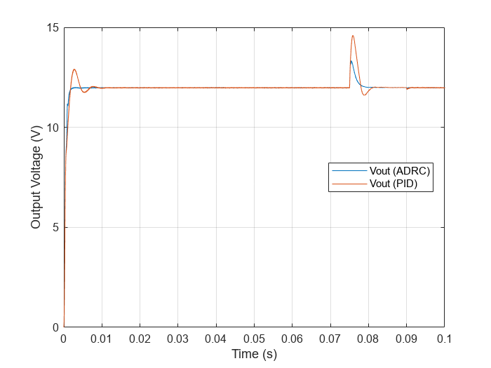
In addition, the ADRC controller works for a wide range of operating points. As a result, retuning is not necessary as with PID controllers. For example, you can compare the performance of the controllers with reference voltage of 12 V.
Set to 12 V and simulate the model.
set_param([mdl,'/Vref'],'Value','12')
set_param(mdl,'SignalLoggingName','pidSim2');
sim(mdl);
Vout_pid2 = getElement(pidSim2,'Output Voltage');
set_param(mdl,'SignalLoggingName','adrcSim2');
set_param([mdl,'/Controller'],'LabelModeActiveChoice','ADRC')
sim(mdl);
Vout_adrc2 = getElement(adrcSim2,'Output Voltage');
Compare the performance.
figure;
plot(Vout_adrc2.Values.Time,Vout_adrc2.Values.Data...
    ,Vout_pid2.Values.Time,Vout_pid2.Values.Data)
grid on
xlabel('Time (s)')
ylabel('Output Voltage (V)')
legend('Vout (ADRC)','Vout (PID)','Location','best')
figure;
plot(Vout_adrc2.Values.Time,Vout_adrc2.Values.Data...
    ,Vout_pid2.Values.Time,Vout_pid2.Values.Data)
grid on
xlim([0.06 0.1])
xlabel('Time (s)')
ylabel('Output Voltage (V)')
legend('Vout (ADRC)','Vout (PID)')

As in the previous scenario, the ADRC controller achieves faster convergence than the PID controller.
You can set the reference voltage to values other than the original 18 V. With easy tuning, the ADRC controller performs much better than the PID controller over a wide range of operating points.
Close the model.
close_system(mdl,0);
References
[1] Lee, S. W. "Practical Feedback Loop Analysis for Voltage-Mode Boost Converter." Application Report No. SLVA633. Texas Instruments. January 2014. www.ti.com/lit/an/slva633/slva633.pdf
See Also
Active Disturbance Rejection Control