Simulation of Bouncing Ball
This example uses two models of a bouncing ball to show different approaches to modeling hybrid dynamic systems with Zeno behavior. Zeno behavior is informally characterized by an infinite number of events occurring in a finite time interval for certain hybrid systems. As the ball loses energy, the ball collides with the ground in successively smaller intervals of time.
Hybrid Dynamic Systems
A bouncing ball model is an example of a hybrid dynamic system. A hybrid dynamic system is a system that involves both continuous dynamics and discrete transitions where the system dynamics can change and the state values can jump. The continuous dynamics of a bouncing ball are given by these equations:


where  is the acceleration due to gravity,
  is the position of the ball, and
  is the velocity. The system has two continuous states: the position
  and the velocity
  .
.
The hybrid system aspect of the model originates from the modeling of a collision of the ball with the ground. If one assumes a partially elastic collision with the ground, then the velocity before the collision,  , and velocity after the collision,
  , can be related by the coefficient of restitution of the ball,
  , as follows:
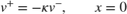
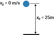
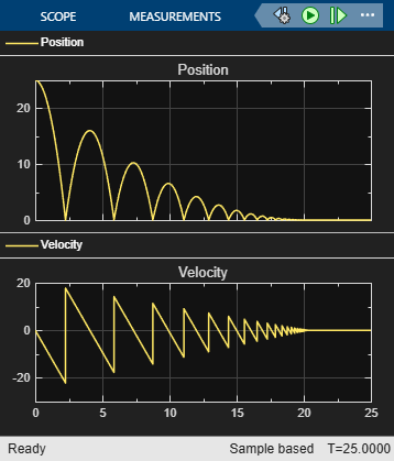
The bouncing ball therefore displays a jump in a continuous state (velocity) at the transition condition,  . The image shows a ball thrown up with a velocity of 0 m/s from a height of 25 m.
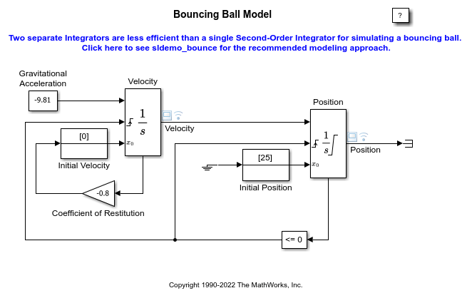
Use Two Integrator Blocks to Model Bouncing Ball
The sldemo_bounce_two_integrators model uses two Integrator blocks to model a bouncing ball. The Integrator block on the left is the velocity integrator modeling the first equation. The Integrator block on the right is the position integrator. Open the Block Parameters dialog box for the position integrator to see that the block has a lower limit of zero. This condition represents the constraint that the ball cannot go below the ground.
The state port of the position integrator and the corresponding comparison result are used to detect when the ball hits the ground and to reset both integrators. The state port of the velocity integrator is used for the calculation of .
To observe the Zeno behavior of the system, modify solver configuration parameters.
To open the Configuration Parameters dialog box, on the Modeling tab, under Setup, click Model Settings.
Select the Solver pane.
Set the Stop time to
25.Click the arrow next to Solver details to view additional solver parameters.
Under Zero-crossing options, set Algorithm to
Nonadaptive.
Simulate the model.
As the ball hits the ground more frequently and loses energy, the simulation exceeds the default Number of consecutive zero crossings limit of 1000.
In the Configuration Parameters dialog box, set Algorithm to Adaptive. The adaptive algorithm introduces a sophisticated treatment for chattering behavior. You can now simulate the system beyond 20 seconds. The chatter of the states between 21 seconds and 25 seconds is still large, and the software issues a warning around 20 seconds.
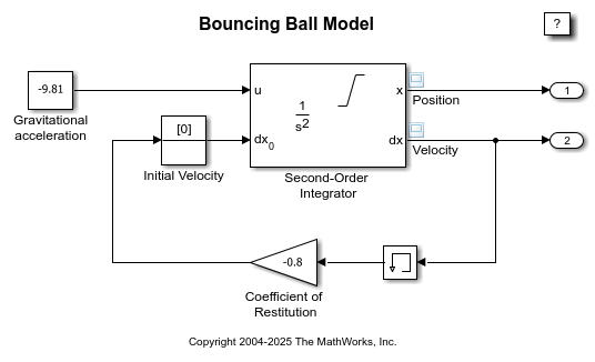
Use Second-Order Integrator Block to Model Bouncing Ball
The sldemo_bounce model uses a single Second-Order Integrator block to model a bouncing ball. In this model, the second equation  is internal to the Second-Order Integrator block. Open the Second-Order Integrator block dialog box and see that has a lower limit of zero. On the Attributes tab, select
 Reinitialize dx/dt when x reaches saturation. This parameter allows you to reinitialize  ( in the bouncing ball model) to a new value when reaches its saturation limit. So, in the bouncing ball model, when the ball hits the ground, its velocity can be set to a different value, such as to the velocity after the impact. Note the loop for calculating the velocity after a collision with the ground. To capture the velocity of the ball just before the collision, the output port of the Second-Order Integrator block and a Memory block are used. is then used to calculate the rebound velocity .
In the Configuration Parameters dialog box, go to the Solver pane.
In Simulation time, set Stop time to
25.Expand Solver details. In Zero-crossing options, set Algorithm to
Nonadaptive.
Simulate the model.
Note that the simulation encounters no problems. You can simulate the model without experiencing excessive chatter after 20 seconds and without setting Algorithm to Adaptive.
Compare Approaches to Modeling Bouncing Ball
You can analytically calculate the exact time  when the ball settles down to the ground with zero velocity by summing the time required for each bounce. This time is the sum of an infinite geometric series given by:
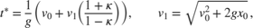
where  and
and  are initial conditions for position and velocity, respectively. The velocity and the position of the ball must be identically zero for
  . The figure shows results from both simulations near . The vertical red line in the plot is for the given model parameters. For
  and far away from , both models produce accurate and identical results. Only a magenta line from the second model is visible in the plot. However, the simulation results from the first model are inexact after . The plot continues to display excessive chattering behavior for . In contrast, the model that uses the Second-Order Integrator block settles to exactly zero for
  .
.
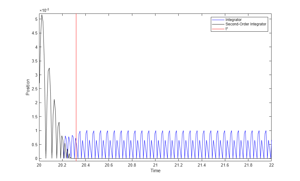
The model that uses the Second-Order Integrator block has superior numerical characteristics compared to the first model because the second differential equation is internal to the Second-Order Integrator block. The block algorithms can leverage this relationship between the two states and use heuristics to clamp down chattering behavior for certain conditions. These heuristics become active when the two states are no longer mutually consistent due to integration errors and chattering behavior. You can thus use physical knowledge of the system to prevent simulations getting stuck in a Zeno state for certain classes of Zeno models.
See Also
Integrator | Second-Order Integrator | Memory