Partition a Model
You can make your model real-time capable by dividing the computational cost for simulation between multiple processors via model partitioning. Computational cost is a measure of the number and complexity of tasks that a central processing unit (CPU) performs per time step during a simulation. A high computational cost can slow simulation execution speed and cause overruns when you simulate in real time on a single CPU.
Typically, you can lower computational costs enough for real-time simulation on a single processor by adjusting model fidelity and solver settings using methods described in Model Preparation Process. However, it is possible that there is no combination of model complexity and solver settings that can make your model real-time capable on a single CPU on your target machine. If your real-time simulation using a single CPU does not run to completion, or if the results from the simulation are not acceptable, partition your model. You can run a partitioned model using a single, multi-core target machine or multiple, single-core target machines.
This example shows you how to partition your model into two discrete subsystems, one that contains the plant, and one that contains the controller, for parallel processing on individual real-time CPUs.
Open the model. At the MATLAB® command prompt, enter
model = 'ssc_hydraulic_actuator_digital_control';
open_system(model)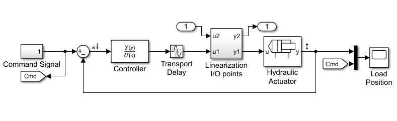
In addition to signal routing and monitoring blocks, the model contains these blocks:
Command Signal — A masked subsystem that generates the input reference signal, r.
Sum — A block that compares the reference signal, r, from the Command Signal block to the output signal, y, from the Hydraulic Actuator to generate the error, x, that is r - y = x.
Controller — A continuous Transfer Fcn block. The Numerator coefficients and Denominator coefficients parameters for this block are specified by the variables
numandden.Transport Delay — A block that simulates time delay for a continuous input signal.
Note
By default, Simulink® Editor hides the automatic block names in model diagrams. To display hidden block names for training purposes, clear the Hide Automatic Block Names check box. For more information, see Configure Model Element Names and Labels.
Linearization I/O — A subsystem that linearizes the model about an operating point.
Hydraulic Actuator — A subsystem that contains the Simscape™ plant model.
Examine the variables in the workspace by clicking each variable in turn.
The variable for sample time, ts =
0.001.The Numerator coefficients parameter, num =
-0.5.The Denominator coefficients parameter, den =
[0.001 1].The variable ClosedLoop =
1.
Simulate the model and open the Load Position scope to examine the results.
sim(model)
open_system([model, '/Load Position'])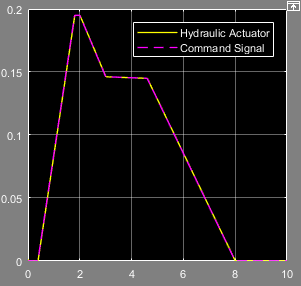
The output from the hydraulic actuator matches the command signal.
Eliminate items that add to the computational cost but which do not affect the results of real-time simulation. In the example model, because the closed loop gain is 1, such items include the Linearization I/O points, In1, and In2 blocks. Delete the three blocks and the lines that interconnect them.
Configure the model for visualization.
Delete the Mux block.
Delete the Goto and From blocks that are named Cmd.
Connect the Load Position Scope block to the output signal from the Hydraulic Actuator.
Add a second Scope block.
Connect the new Scope block to the unconnected connection line from the Command Signal.
Change the name of the new Scope block to
Reference.
Replace the Transport Delay block with a Unit Delay block.
Delete the Transport Delay block and the open ended connection line that is connected to the outport of the block.
Add the Unit Delay block from the Simulink Discrete library and connect it to the input port of the Hydraulic Actuator Subsystem.
For the Sample time (-1 for inherited) parameter of the Unit Delay block, specify
ts.
Replace the Controller block with a Discrete Transfer Fcn block from the Simulink Discrete library.
Delete the Controller block.
Click in the model window and enter
discrete transfer
                                    fcn
. When the dropdown menu that contains the block appears, clickDiscrete Transfer Fcn.Connect the new block to the open-ended connection line from the Sum block.
Connect the outport of the new block to the inport of the Unit Delay block.
Specify parameters for the discrete controller using a Tustin transformation of the original, continuous transfer function.
At the MATLAB command line, save new variables based on the original coefficients:
k = num; alpha = den(1,1);
For the Discrete Transfer Fcn block Numerator parameter, specify
[k*ts k*ts].For the Denominator parameter, specify
[2*alpha+ts ts-2*alpha].For the Sample time (-1 for inherited) parameter, specify
ts.
Provide digital sampling for continuous time measurements using Zero-Order Hold blocks.
Add Zero-Order Hold blocks to both signals that are input to the Sum block.
For the Sample time (-1 for inherited) parameter of both Zero-Order Hold blocks, specify
ts.
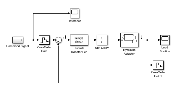
Connect the blocks as shown in the figure.
Simulate the model and open the Load Position scope to see how the modifications affect the results.
sim(model) open_system([model, '/Load Position'])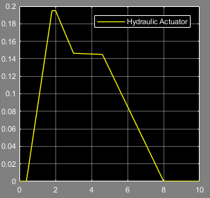
The output from the hydraulic actuator matches the original results.
Configure the solvers.
To configure the global solver, open the model configuration parameters, and in the Solver pane:
Set the solver Type to
Fixed-step.Set the Solver to
discrete (no continuous states).Specify
tsfor the Fixed-step size (fundamental sample time) parameter.Click OK.
To configure the local solver, open the Hydraulic Actuator subsystem and update these parameters for the Solver Configuration block:
Select the option to Use local solver.
Specify
tsfor the Sample time.Select the option to Use fixed-cost runtime consistency iterations.
Click OK.
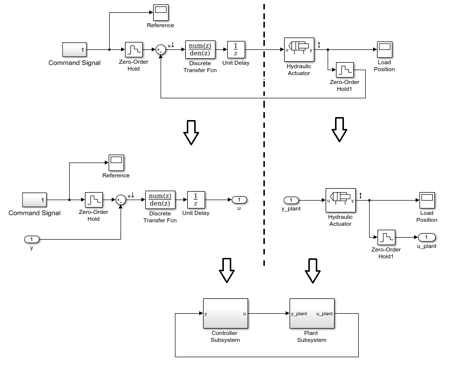
Partition the model into two subsystems:
Create a subsystem that contains these blocks:
Command Signal
Reference
Zero-Order Hold
Sum
Discrete Transfer
                                Fcn
Unit Delay
Label the subsystem
Controller Subsystem.Open the Controller Subsystem.
Rename the Out1 Outport block as
u.Rename the In1 Inport block as
y.Navigate to the top model.
Create a second subsystem that contains these blocks:
Hydraulic Actuator
Zero-Order Hold1
Load Position
Label the subsystem
Plant Subsystem.Open the Plant Subsystem.
Rename the Out1 Outport block as
u_plant.Rename the In1 Inport block as
y_plant.To see the partitioned subsystems, navigate to the top model.
This model is partitioned for concurrent execution. To learn how to add tasks, and map individual tasks to partitions, see Partition Your Model Using Explicit Partitioning.
See Also
Discrete Transfer Fcn | Unit Delay | Zero-Order Hold
Topics
- Determine Step Size
- Estimate Computation Costs
- Reduce Computation Costs
- Implicit and Explicit Partitioning of Models
- Multicore Programming with Simulink