pulstran

Pulse train

Syntax

y = pulstran(t,d,func)

y = pulstran(t,d,func,fs)

y = pulstran(t,d,p)

y = pulstran(___,intfunc)

Description

y = pulstran(t,d,func) generates a pulse train based on samples of a continuous function, func.

y = pulstran(t,d,func,fs) uses a sample rate of fs.

y = pulstran(t,d,p) generates a pulse train that is the sum of multiple delayed interpolations of the prototype pulse in vector p.

y = pulstran(___,intfunc) specifies alternative interpolation methods. See interp1 for a list of available methods. You can use this parameter with any of the previous input syntaxes.

Examples

Periodic Rectangular Pulse

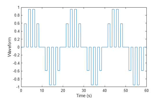
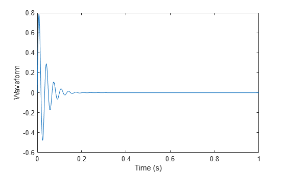
This example generates a pulse train using the default rectangular pulse of unit width. The repetition frequency is 0.5 Hz, the signal length is 60 s, and the sample rate is 1 kHz. The gain factor is a sinusoid of frequency 0.05 Hz.

t = 0:1/1e3:60;
d = [0:2:60;sin(2*pi*0.05*(0:2:60))]';
x = @rectpuls;
y = pulstran(t,d,x);

plot(t,y)
hold off
xlabel('Time (s)')
ylabel('Waveform')

Asymmetric Sawtooth Waveform

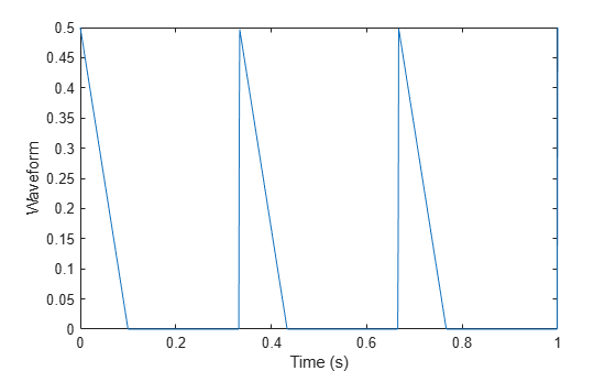
This example generates an asymmetric sawtooth waveform with a repetition frequency of 3 Hz. The sawtooth has width 0.2 s and skew factor –1. The signal length is 1 s, and the sample rate is 1 kHz. Plot the pulse train.

fs = 1e3;
t = 0:1/1e3:1;
d = 0:1/3:1;   
x = tripuls(t,0.2,-1);
y = pulstran(t,d,x,fs);

plot(t,y)
hold off
xlabel('Time (s)')
ylabel('Waveform')

Periodic Gaussian Pulse

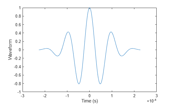
Plot a 10 kHz Gaussian RF pulse with 50% bandwidth, sampled at a rate of 10 MHz. Truncate the pulse where the envelope falls 40 dB below the peak.

fs = 1e7;
tc = gauspuls('cutoff',10e3,0.5,[],-40); 
t = -tc:1/fs:tc; 
x = gauspuls(t,10e3,0.5); 

plot(t,x)
xlabel('Time (s)')
ylabel('Waveform')

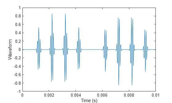
The pulse repetition frequency is 1 kHz, the sample rate is 50 kHz, and the pulse train length is 25 ms. The gain factor is a sinusoid of frequency 0.1 Hz.

ts = 0:1/50e3:0.025;
d = [0:1/1e3:0.025;sin(2*pi*0.1*(0:25))]';
y = pulstran(ts,d,x,fs);

Plot the periodic Gaussian pulse train.

plot(ts,y)
xlim([0 0.01])
xlabel('Time (s)')
ylabel('Waveform')

Custom Pulse Trains

Write a function that generates custom pulses consisting of a sinusoid damped by an exponential. The pulse is an odd function of time. The generating function has a second input argument that specifies a single value for the sinusoid frequency and the damping factor. Display a generated pulse, sampled at 1 kHz for 1 second, with a frequency and damping value, both equal to 30.

fnx = @(x,fn) sin(2*pi*fn*x).*exp(-fn*abs(x));

ffs = 1000;
tp = 0:1/ffs:1;

pp = fnx(tp,30);

plot(tp,pp)
xlabel('Time (s)')
ylabel('Waveform')

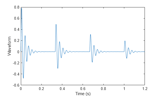
Use the pulstran function to generate a train of custom pulses. The train is sampled at 2 kHz for 1.2 seconds. The pulses occur every third of a second and have exponentially decreasing amplitudes.

Initially specify the generated pulse as a prototype. Include the prototype sample rate in the function call. In this case, pulstran replicates the pulses at the specified locations.

fs = 2e3;
t = 0:1/fs:1.2;

d = 0:1/3:1;
dd = [d;4.^-d]';

z = pulstran(t,dd,pp,ffs);

plot(t,z)
xlabel('Time (s)')
ylabel('Waveform')

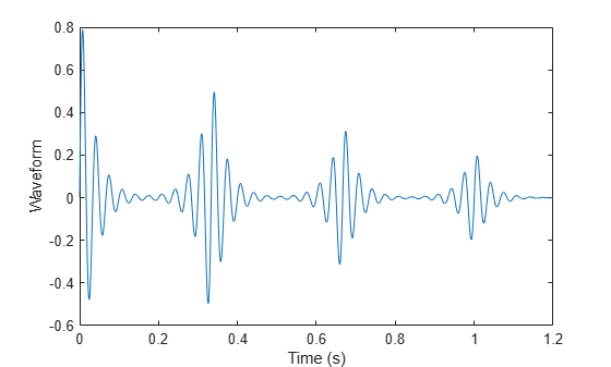
Generate the pulse train again, but now use the generating function as an input argument. Include the frequency and damping parameter in the function call. In this case, pulstran generates the pulse so that it is centered about zero.

y = pulstran(t,dd,fnx,30);

plot(t,y)
xlabel('Time (s)')
ylabel('Waveform')

Change Interpolation Method with Custom Pulse

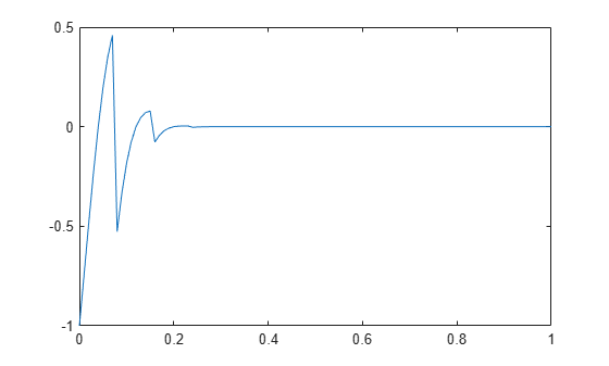
Write a function that generates a custom exponentially decaying sawtooth waveform of frequency 0.25 Hz. The generating function has a second input argument that specifies a single value for the sawtooth frequency and the damping factor. Display a generated pulse, sampled at 0.1 kHz for 1 second, with a frequency and damping value equal to 50.

fnx = @(x,fn) sawtooth(2*pi*fn*0.25*x).*exp(-2*fn*x.^2);

fs = 100;
t = 0:1/fs:1;

pp = fnx(t,50);

plot(t,pp)

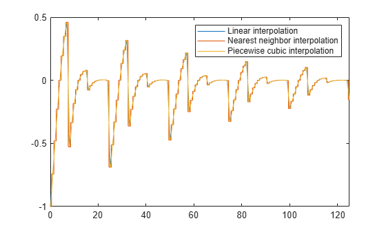
Use the pulstran function to generate a train of custom pulses. The train is sampled at 0.1 kHz for 125 seconds. The pulses occur every 25 seconds and have exponentially decreasing amplitudes.

Specify the generated pulse as a prototype. Generate three pulse trains using the default linear interpolation method, nearest neighbor interpolation and piecewise cubic interpolation. Compare the pulse trains on a single plot.

d = [0:25:125; exp(-0.015*(0:25:125))]';
ffs = 100;
tp = 0:1/ffs:125;

r = pulstran(tp,d,pp);
y = pulstran(tp,d,pp,'nearest');
q = pulstran(tp,d,pp,'pchip');


plot(tp,r)
hold on
plot(tp,y)
plot(tp,q)
xlim([0 125])
legend('Linear interpolation','Nearest neighbor interpolation','Piecewise cubic interpolation')
hold off

Input Arguments

t — Time values

vector

Time values at which func is evaluated, specified as a vector.

d — Offset

row vector | two-column matrix

Offset removed from the values of the array t, specified as a real vector. You can apply an optional gain factor to each delayed evaluation by specifying d as a two-column matrix, with offset defined in column 1 and associated gain in column 2. If you specify d as a row vector, the values are interpreted as delays only.

func — Continuous function

'rectpuls' | 'gauspuls' | 'tripuls' | function handle

Continuous function used to generate a pulse train based on its samples, specified as 'rectpuls', 'gauspuls', 'tripuls', or a function handle.

If you use func as a function handle, you can pass the function parameters as follows:

y = pulstran(t,d,'gauspuls',10e3,0.5); 

This creates a pulse train using a 10 kHz Gaussian pulse with 50% bandwidth.

p — Prototype pulse

vector

Prototype function, specified as a vector. The interval of p is given by [0,(length(p)-1)/fs], and its samples are identically zero outside this interval. By default, linear interpolation is used for generating delays.

fs — Sample rate

1 (default) | real scalar

Sample rate in Hz, specified as a real scalar.

intfunc — Interpolation method

'linear' (default) | 'nearest' | 'next' | 'previous' | 'pchip' | 'cubic' | 'v5cubic' | 'makima' | 'spline'

Interpolation method, specified as one of the options in this table.

Method	Description	Continuity	Comments
'linear'	Linear interpolation. The interpolated value at a query point is based on linear interpolation of the values at neighboring grid points in each respective dimension. This is the default interpolation method.	C0	Requires at least 2 points Requires more memory and computation time than nearest neighbor
'nearest'	Nearest neighbor interpolation. The interpolated value at a query point is the value at the nearest sample grid point.	Discontinuous	Requires at least 2 points Modest memory requirements Fastest computation time
'next'	Next neighbor interpolation. The interpolated value at a query point is the value at the next sample grid point.	Discontinuous	Requires at least 2 points Similar memory requirements and computation time as 'nearest'
'previous'	Previous neighbor interpolation. The interpolated value at a query point is the value at the previous sample grid point.	Discontinuous	Requires at least 2 points Similar memory requirements and computation time as 'nearest'
'pchip' or 'cubic'	Shape-preserving piecewise cubic interpolation. The interpolated value at a query point is based on a shape-preserving piecewise cubic interpolation of the values at neighboring grid points.	C1	Requires at least 4 points Requires more memory and computation time than 'linear'
'v5cubic'	Cubic convolution used in MATLAB® 5.	C1	Points must be uniformly spaced.
'makima'	Modified Akima cubic Hermite interpolation. The interpolated value at a query point is based on a piecewise function of polynomials with a degree of at most three. The Akima formula is modified to avoid overshoots.	C1	Requires at least 2 points Produces fewer undulations than 'spline', but does not flatten as aggressively as 'pchip' Computation is more expensive than 'pchip', but typically less than 'spline' Memory requirements are similar to those of 'spline'
'spline'	Spline interpolation using not-a-knot end conditions. The interpolated value at a query point is based on a cubic interpolation of the values at neighboring grid points in each respective dimension.	C2	Requires at least 4 points Requires more memory and computation time than 'pchip'

Output Arguments

y — Pulse train

vector

Pulse train generated by the function, returned as a vector.

Extended Capabilities

C/C++ Code Generation

Generate C and C++ code using MATLAB® Coder™.

Usage notes and limitations:

• The pulse function can only be tripuls, rectpuls, or gauspuls.

• If you specify a custom pulse instead of a pulse function, then the limitations for interp1 apply.

Version History

Introduced before R2006a