Using Multiple-Edge Response (MER) to Represent Nonlinear Systems
This example highlights the concepts of multiple-edge response (MER) representation and lays the ground work that is built upon in other examples which explore how to apply AMI equalization to signals.
To accurately and reliably calculate the bit error rate (BER) of a system, signal integrity analysis often requires simulating millions of bits of waveforms. Circuit simulators like HSPICE or IsSpice4 generate the most accurate waveforms, but they operate too slowly to efficiently produce millions of bits. If you assume the channel, transmitters, and receivers are linear and time-invariant (LTI), then you can fully characterize the system with an impulse response. You can easily calculate impulse responses from S-parameters or through quick circuit simulations. With an LTI system, you can perform frequency domain analysis, use fast convolution techniques like IBIS-AMI to quickly generate long waveforms, and apply analytic methods such as peak distortion analysis and statistical eye analysis to estimate BER at very low probabilities.
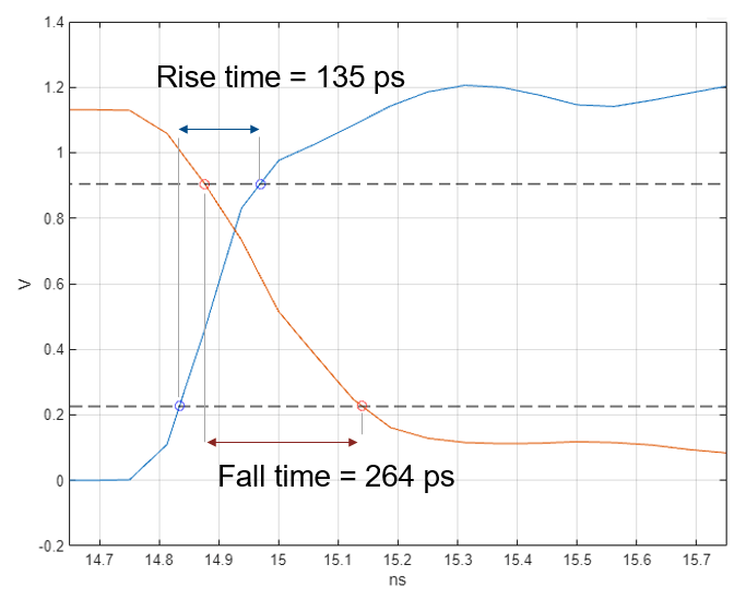
However, when the system behaves nonlinearly, these traditional signal integrity tools cannot accurately or reliably determine system performance. While the LTI assumption holds for many differential communication links, most single-ended communication links exhibit several nonlinearities that complicate analysis. For example, pseudo-open drain transceiver architectures, commonly used in high-speed DDR interfaces, produce rise times that differ significantly from fall times. Additionally, the output impedance of these transmitters depends on the driving state, causing any channel reflections to bounce off the transmitter with a reflection coefficient that varies according to the driving data pattern. An illustration of a system with asymmetrical rise and fall times is shown below:
MER analysis addresses the challenges of modeling nonlinear systems by extending system characterization from a single impulse response to a set of edge responses. By assuming each edge response is conditionally LTI, MER analysis captures the full system behavior, enabling fast-convolution waveform generation and statistical eye analysis.
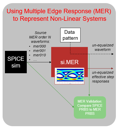
An overview of the example is illustrated below where the SPICE simulation provides the source waveforms from which si.MER calculates the effective step responses needed to reconstruct an arbitrary data pattern and calculate nonlinear statistical eye diagrams. Validation of the MER representation is obtained by comparing the MER reconstruction of a short data pattern with the SPICE simulation of the same data pattern.
Dual Edge Response or MER Order 1
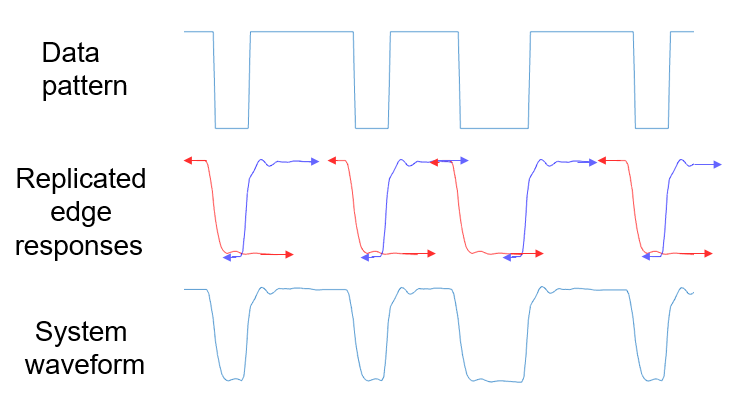
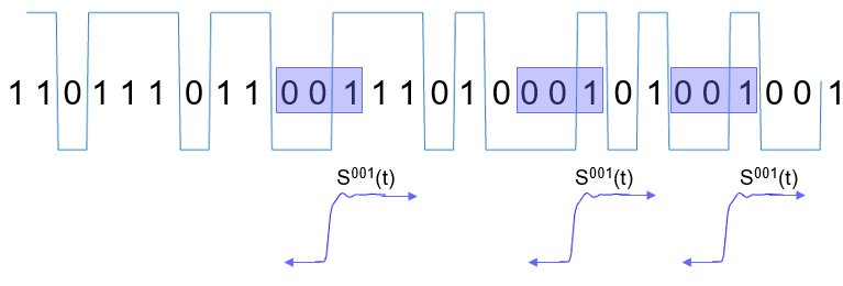
How can you characterize a nonlinear system that you cannot represent with an impulse response? If you know the system exhibits distinct behaviors for rising and falling edges, you can reasonably choose to represent it with separate rising and falling step responses. Researchers have called this approach the dual edge response [1], but following [2-3], you can generalize the analysis and refer to it as MER order 1. To conceptualize this, consider how you can reconstruct a given data pattern by combining the rising and falling edge responses to generate the system waveform. The illustration below shows the falling edge responses in red and the rising edge response in blue. Red and blue arrows attached to each side of the edge responses indicate that these responses theoretically extend indefinitely. This representation treats the system as conditionally-LTI: when the system transitions from a low to high state, the rising edge response locally describes the system behavior, and the falling edge response does so for high-to-low transitions. Using this conditional-LTI model, you can apply superposition and sum the time-shifted edge responses (in red and blue) to estimate how the system responds to a given stimulus data pattern. These edge responses are the effective edge responses you encounter later.
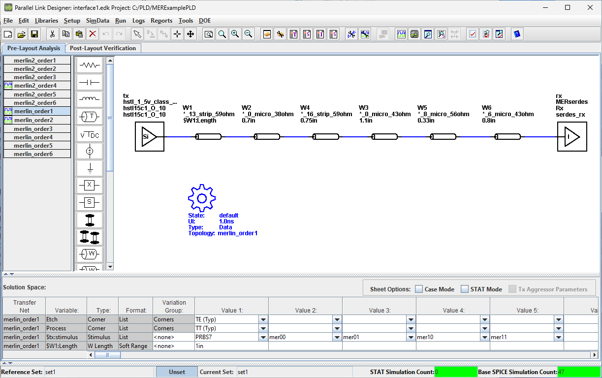
The following image of a Parallel Link Designer project contains a system with a nonlinear transmitter, a short reflective channel, and an ideal receiver. The simple NRZ transmitter has asymmetric rise and fall time as well as an output impedance that is dependent on the driving voltage of the transmitter. This system will allow for a demonstration of the capabilities and power of MER analysis. Each sheet contains a sweep of the stimulus pattern which includes a PRBS 7 pattern and MER source patterns.
The following MATLAB code extracts the required source waveforms from the Parallel Link Designer project. The code downloads and simulates the example project folder, MERExamplePLD, if it does not exist. Simulation may take several minutes. You can speed up the simulation by enabling the parallel options. The MER representation is validated by comparing the MER reconstructed waveform with an output circuit level simulation waveform of the same data pattern.
% Define the MER order
Order = 1;

% Define the samples per symbol for resampling the simulation data
SamplesPerSymbol = 16;

% Define Parallel Link Designer (PLD) project path
ProjectPLD = fullfile(pwd,'MERExamplePLD');

% Define the PLD sheet name
sheetname = sprintf('merlin_order%i',Order);

% Extract PLD data and prepare for AMI simulations.  If the PLD project
% MERExamplePLD doesn't exist yet, then it will be downloaded from the Kit
% repository and simulated.
simDataOrder1 = spice2mer(ProjectPLD, sheetname, Order, SamplesPerSymbol);

% Create the MER object with the order 1 simulation data
RepresentationMER1 = si.MER(...
    'Order', Order,...
    'Modulation', 2,...
    'SamplesPerSymbol', SamplesPerSymbol,...
    'PlotAxis', 'Seconds',...
    'SymbolTime', simDataOrder1.SymbolTime,...
    'Specification', 'Wave',...
    'SourceWaves', simDataOrder1.PatternWave,...
    'SourceWavesPattern', simDataOrder1.PatternMat,...
    'ApplyStepSelfConsistency',true,...
    'ReferenceWave',simDataOrder1.ReferenceWave,...
    'ReferenceWavePattern',simDataOrder1.ReferencePattern);
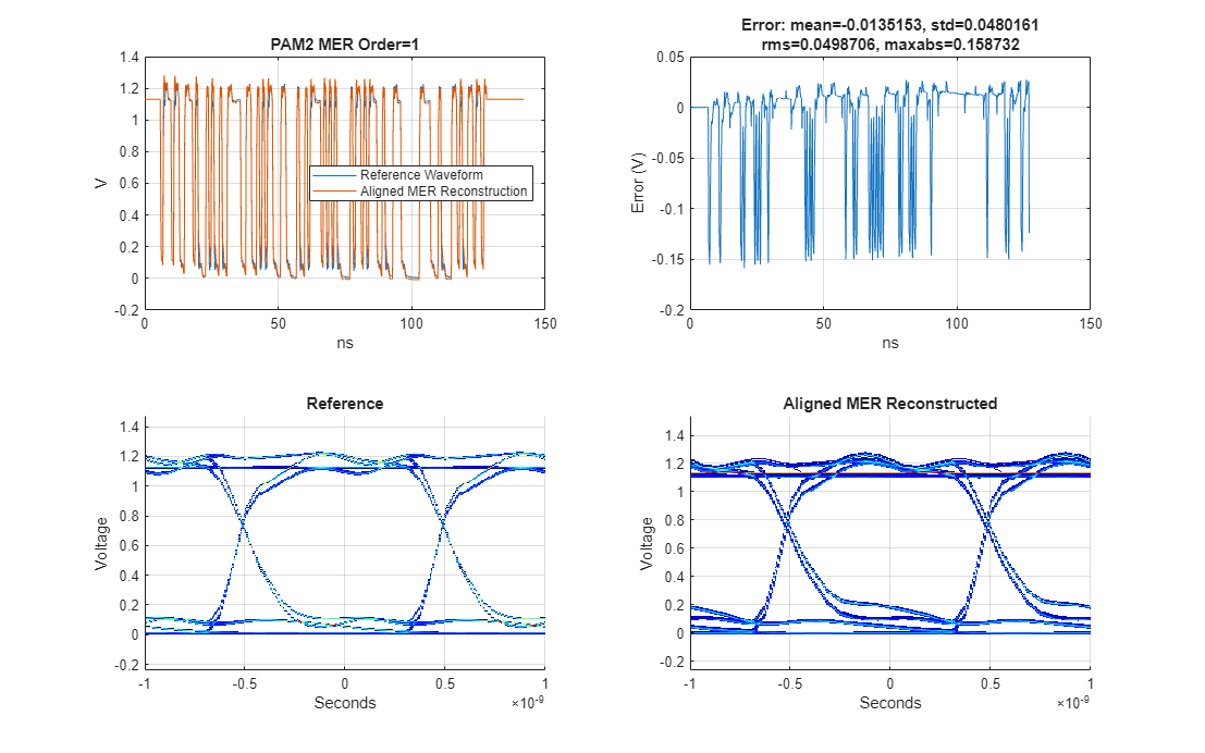
The plotValidation method displays four plots:
1) the reference circuit simulated PRBS waveform with the aligned MER reconstructed waveform together,
2) the difference between the reference and reconstructed waveform,
3) the reference waveform eye diagram, and
4) the reconstructed waveform eye diagram.
For this case, the maximum difference between the reference waveform and the MER order 1 reconstructed waveform is more than 150 mV.
% Visualize validation results
h1 = figure('IntegerHandle','off');
plotValidation(RepresentationMER1)
set(h1,'Units','normalized','Position',[ 0 0 1 1]);
The following short report also returns the mean error, the standard deviation of the error, the root-mean-square of the error, and the maximum absolute error in Volts.
% Display validation report metrics
disp(RepresentationMER1.ValidationResults.Report)
Error: mean=-0.0135153, std=0.0480161, rms=0.0498706, max=0.158732
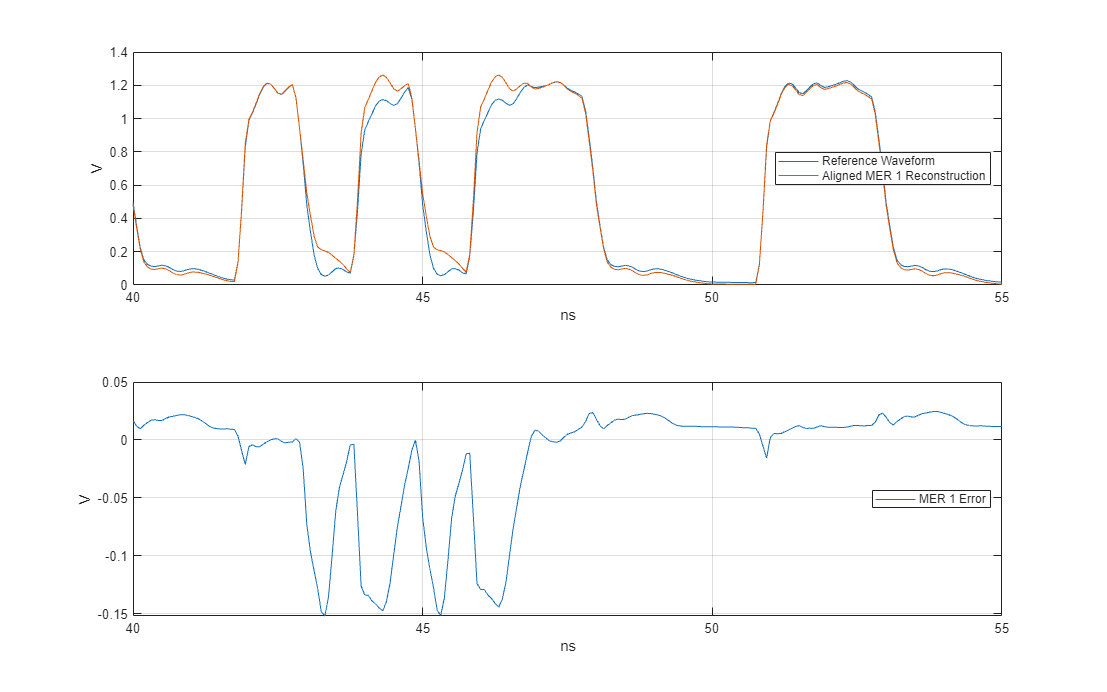
The following figure zooms in on the time axis to compare the reference waveform, the reconstructed waveform, and the resulting error. This view highlights several interesting characteristics of the MER order 1 representation. When an edge appears relatively isolated, the MER order 1 representation accurately matches the desired reference waveform behavior. However, when other transitions immediately preceded the edge, the MER order 1 representation produces large errors. If these representation errors arise from multiple reflections within the channel and a transmitter exhibiting time-variant output impedance, then using a higher order MER representation could provide a more accurate model.
% Setup the time vectors for plotting
[trefvec1,xunit1,tscale1]=SetupTimeVector(RepresentationMER1,length(RepresentationMER1.ReferenceWave));
tsynvec1 = tscale1*(0:length(RepresentationMER1.WaveAligned)-1);
tdiffvec1 = tscale1*(0:length(RepresentationMER1.WaveDifference)-1);

% Plot the reference and reconstructed waveforms
h2 = figure('IntegerHandle','off');
tiledlayout(2,1)
ax2(1) = nexttile;
plot(trefvec1,RepresentationMER1.ReferenceWave,...
tsynvec1,RepresentationMER1.WaveAligned)
ylabel('V')
xlabel(xunit1)
grid on
hLeg = legend('Reference Waveform','Aligned MER 1 Reconstruction',...
'location','east');
hLeg.ItemHitFcn = @si.MER.ToggleLineVisibility;

% Plot difference waveform
ax2(2) = nexttile;
plot(tdiffvec1,RepresentationMER1.WaveDifference)
legend('MER 1 Error','location','east');
grid on
ylabel('V')
xlabel(xunit1)

linkaxes(ax2,'x')
set(h2,'Units','normalized','Position',[ 0 0 1 1]);

% Zoom in
xlim([40 55])
MER Order 2 Representation
Whereas MER order 1 representation utilized a single rising and a single falling edge responses to model the system, MER order 2 representation augments the order 1 edge responses with some additional effective step responses which are pre-conditioned on prior data patterns. Collectively these effective edge responses can better model behavior of the system due to nonlinear and time-variant behavior of the transmitter. A thorough description of the creation of these effective edge responses from circuit simulated data is provided in the section Appendix A: Source Waveforms and Effective Edge Responses. The following discussion offers a more conceptual and less mathematical perspective on effective edge responses.
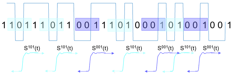
MER order 2 uses four effective step responses: , , and . The waveform is the rising edge response given that the previous two symbols are 00 and is equivalent to the MER order 1 rising edge response. is the rising edge response given that the previous two symbols are 10. is the falling edge response given that the previous two symbols are 11 and is equivalent to the MER order 1 falling edge response. is the falling edge response given the previous two symbols are 01.
The following illustration demonstrates how to use the MER order 2 effective step responses to reconstruct an arbitrary data pattern. For each rising or falling edge in the pattern, match it with the corresponding effective edge response. Small arrows at the start and end of each step response indicate that these responses extend indefinitely. Begin by identifying the edges in the data pattern.
Next, identify the rising edges in the data pattern.
Then identify the falling edges in the data pattern.
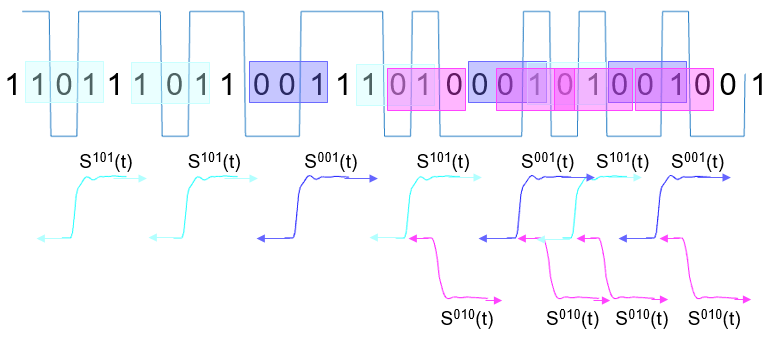
And lastly, identify the falling edges in the data pattern.
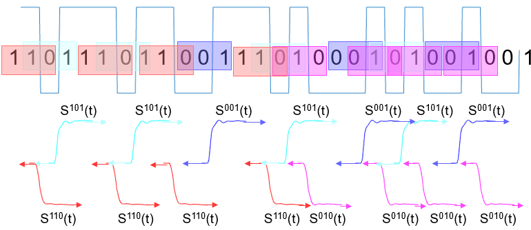
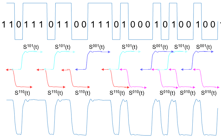
Then sum these shifted and replicated edge responses to construct the non-LTI system waveform.
The MATLAB code below reads in the circuit simulated MER order 2 source waveforms, creates the MER MATLAB object and shows how the order 2 representation improves on the order 1 representation.
% Define the MER order
Order = 2;

% Define Parallel Link Designer sheet name
sheetname = sprintf('merlin_order%i',Order);

% Extract simulation data
simDataOrder2 = spice2mer(ProjectPLD,sheetname, Order, SamplesPerSymbol);

% Create MER object
RepresentationMER2 = si.MER(...
    'Order', Order,...
    'Modulation', 2,...
    'SamplesPerSymbol', SamplesPerSymbol,...
    'PlotAxis', 'Seconds',...
    'SymbolTime', simDataOrder2.SymbolTime,...
    'Specification', 'Wave',...
    'SourceWaves', simDataOrder2.PatternWave,...
    'SourceWavesPattern', simDataOrder2.PatternMat,...
    'ApplyStepSelfConsistency',true,...
    'ReferenceWave',simDataOrder2.ReferenceWave,...
    'ReferenceWavePattern',simDataOrder2.ReferencePattern);
Utilize the plotValidation method for a quick summary of the MER's ability to match the reference waveform from both a waveform and an eye diagram perspective.
% Visualize validation plots comparing reference waveform with MER
% reconstructed waveform
h3 = figure('IntegerHandle','off');
plotValidation(RepresentationMER2)
set(h3,'Units','normalized','Position',[ 0 0 1 1]);
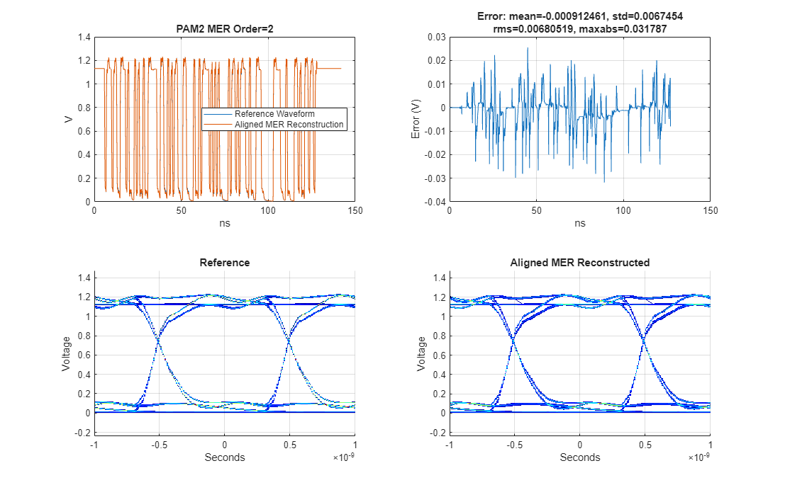
% Display validation report metrics
disp(RepresentationMER2.ValidationResults.Report)
Error: mean=-0.000912461, std=0.0067454, rms=0.00680519, max=0.031787
Before comparing the order 1 and order 2 MER representations, ensure that their reference waveforms are identical.
% Validate that the MER order 1 and 2 reference waveforms are the same
isequal(RepresentationMER1.ReferenceWave,RepresentationMER2.ReferenceWave)
ans = logical
1
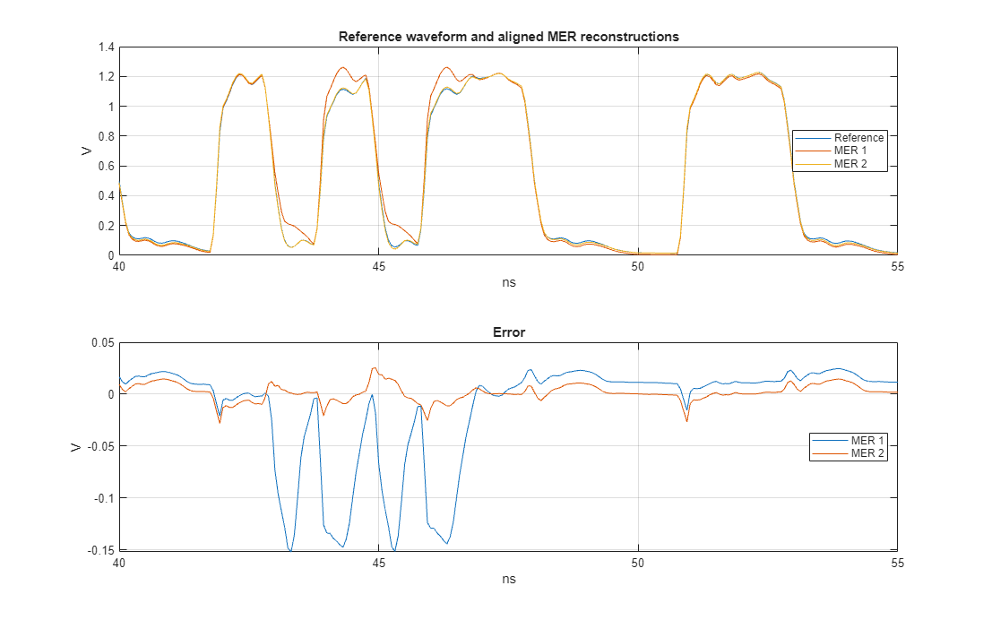
Directly compare the reference waveform and the order 1 and order 2 MER reconstructed waveforms. Note how the order 2 waveform representation greatly improved upon the order 1 waveform representation in comparison to the reference waveform. The maximum error for order 1 is about 159 mV and the maximum error for order 2 is about 32 mV. Increasing the MER order usually can reduce the systematic error magnitude but requires a tradeoff of computational complexity with accuracy. The error you are willing to tolerate will be driven by the needs of the analysis, for instance, trend analysis, which attempts to determine the relative impact of a design parameter, can tolerate a larger analysis error than model correlation analysis which typically requires better model accuracy. This example tolerates a maximum error on the order of 15 to 30 mV.
% Generate time vectors for zoomed-in validation plots
[trefvec2,xunit2,tscale2]=SetupTimeVector(RepresentationMER2,length(RepresentationMER2.ReferenceWave));
tsynvec2 = tscale2*(0:length(RepresentationMER2.WaveAligned)-1);
tdiffvec2 = tscale2*(0:length(RepresentationMER2.WaveDifference)-1);

% Compare reference waveform to MER reconstructed waveforms
h4 = figure('IntegerHandle','off');
tiledlayout(2,1)
ax(1) = nexttile;
plot(trefvec1,RepresentationMER1.ReferenceWave,...
tsynvec1,RepresentationMER1.WaveAligned,...
tsynvec2,RepresentationMER2.WaveAligned)
title('Reference waveform and aligned MER reconstructions')
ylabel('V')
xlabel(xunit1)
grid on
hLeg = legend('Reference','MER 1','MER 2','location','east');
hLeg.ItemHitFcn = @si.MER.ToggleLineVisibility;

ax(2) = nexttile;
plot(tdiffvec1,RepresentationMER1.WaveDifference,...
tdiffvec2,RepresentationMER2.WaveDifference)
title('Error')
ylabel('V')
xlabel(xunit1)
grid on
hLeg2 = legend('MER 1','MER 2','location','east');
hLeg2.ItemHitFcn = @si.MER.ToggleLineVisibility;

linkaxes(ax,'x')
set(h4,'Units','normalized','Position',[ 0 0 1 1]);

xlim([40 55])
MER Statistical Eye Analysis
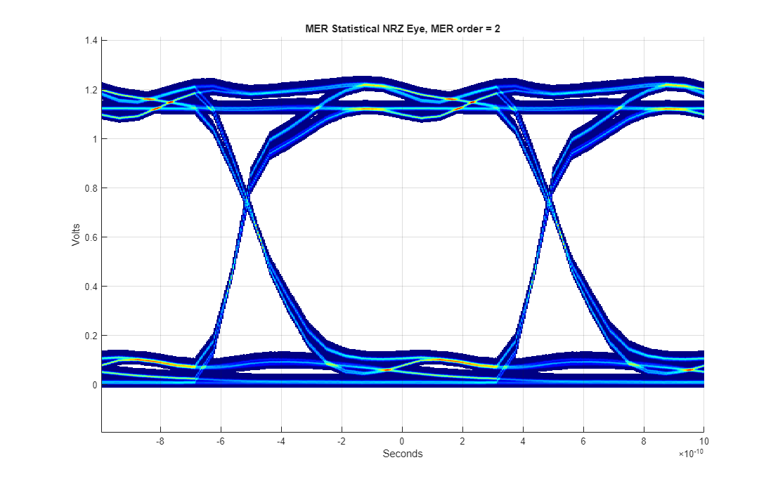
With MER order 2, you can achieve a more accurate representation of the non-LTI system and can apply advanced statistical MER eye analysis to predict system performance at extremely low BER values. Use the plotStateye method to display the statistical eye diagram.
h5 = figure('IntegerHandle','off');
plotStateye(RepresentationMER2)
set(h5,'Units','normalized','Position',[ 0 0 1 1]);
Conclusion
This example demonstrates how effectively MER representation approach models NRZ transmitters that exhibit asymmetrical rise and fall times, as well as output impedance variation dependent on the driver state. MER representation offers a conditionally-LTI approach to modeling nonlinear and time-variant wired systems. A complete representation of the non-LTI system behavior is achieved through a set of effective step responses, each of which is conditioned on the prior data pattern. Higher-order MER representations capture greater data pattern depth and can result in more accurate models. By conditioning the effective step responses on the prior data pattern, higher-order MER representations capture greater data pattern depth. Collectively, these effective edge responses complete the representation space, enabling a fast convolution approach to generate accurate non-LTI time-domain waveforms and perform non-LTI statistical eye estimation. Validate the MER representation by comparing the reconstructed MER waveform to the circuit-level simulation output waveform for a long bit pattern, such as a PRBS 7 sequence.
Increasing the MER order improves the accuracy of the representation, but it also requires more circuit simulation characterization waveforms. The number of required source waveforms grows exponentially as the MER order increases. Eventually, increasing the MER order will no longer enhance accuracy, as it will reach the noise floor of the MER representation. The source of the MER representation noise floor could be due to the error calculation itself due to the alignment and resampling of the waveform or it could be an indication of some other type of systematic uncertainty of the analysis.
The next examples — Multiple-Edge Response (MER) for AMI Statistical Nonlinear System Analysis and Multiple-Edge Response (MER) for AMI Fast Time-Domain Nonlinear System Simulation— show how to incorporate AMI models into MER analysis for generating equalized time domain waveforms and equalized statistical eye diagrams to assess system performance.
Appendix A: Source Waveforms and Effective Edge Responses
MER uses the system's effective edge and step responses to reconstruct non-LTI system waveforms from arbitrary data patterns and to perform non-LTI statistical eye analysis. These effective edge responses depend on the symbols that immediately precede each rising or falling edge.
MER Order 1 Source Waveforms and Effective Edge Responses
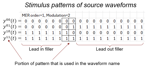
NRZ MER order 1 calls for four source waveforms generated from a circuit simulator. These are all patterns of depth "order + 1". The pattern is extended by repeating the first or last symbol in the pattern.
These four source waveforms are combined into effective step responses as follows:
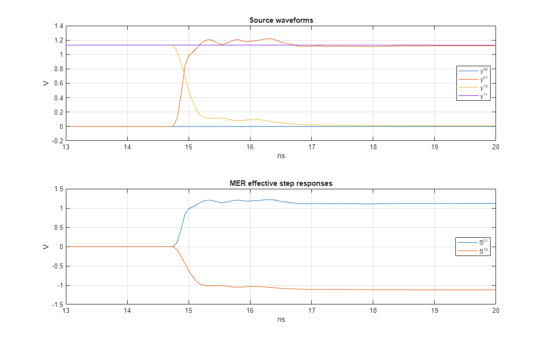
The waveforms and are trivial but are included for completeness. Visualize these responses with plotInputs method. While the effective step responses calculations for MER order 1 are straightforward, generalizing these calculations for higher-order MER allows us to condition the edge responses on the prior data pattern.
h6 = figure('IntegerHandle','off');
plotInputs(RepresentationMER1)
set(h6,'Units','normalized','Position',[ 0 0 1 1]);
xlim([13 20])
MER Order 2 Source Waveforms and Effective Edge Responses
For NRZ MER order 2 source waveforms, you need to include all NRZ patterns of depth "order + 1", which means generating the binary patterns from 0 to 7, as illustrated below. By repeating the first and last symbol of each pattern, you ensure that any reflections or transients have time to diminish before the simulation finishes.
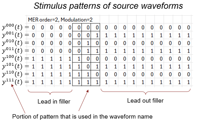
These eight source waveforms are combined into effective step responses as follows:
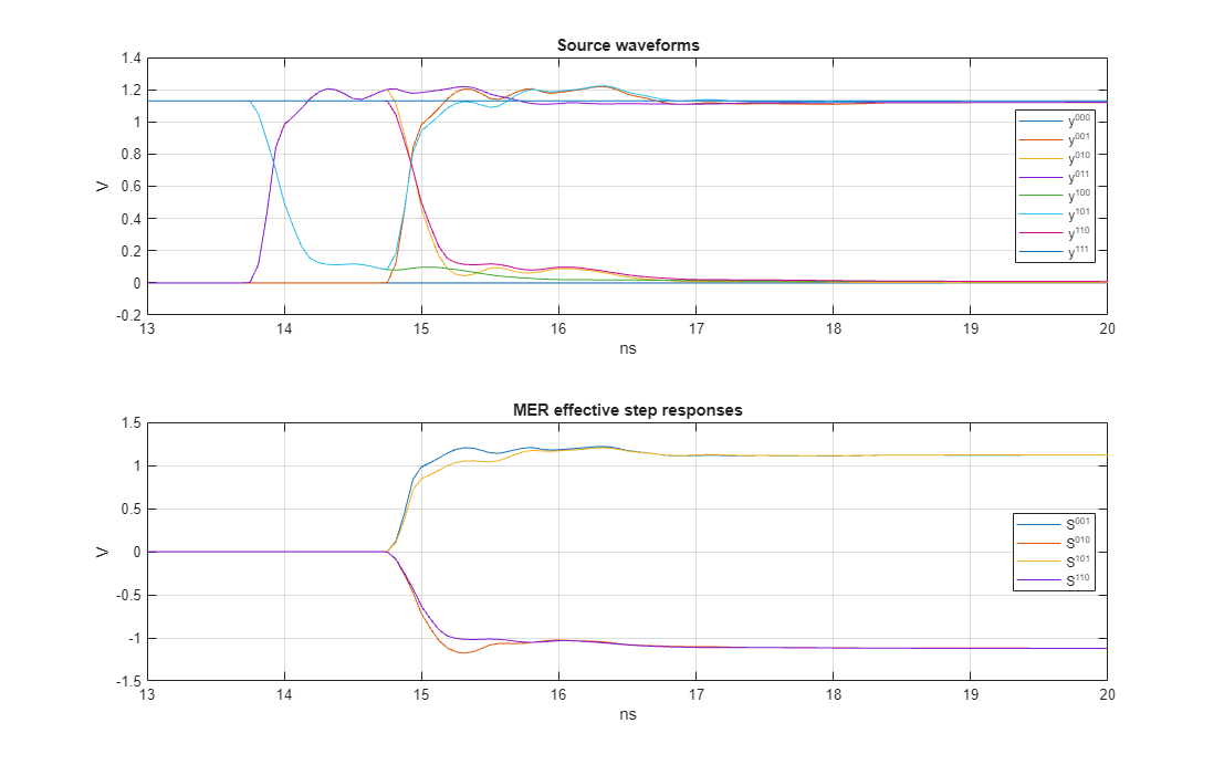
Subtract to remove the effect of prior symbols from the effective step response. The source waveforms and the resulting effective step responses appear below. Notice that the four effective step responses are distinct from one another, illustrating how they span a unique representation space. As a result, higher-order MER representations should deliver more accurate waveform reconstruction than lower-order representations.
h7 = figure('IntegerHandle','off');
plotInputs(RepresentationMER2)
set(h7,'Units','normalized','Position',[ 0 0 1 1]);
xlim([13 20])
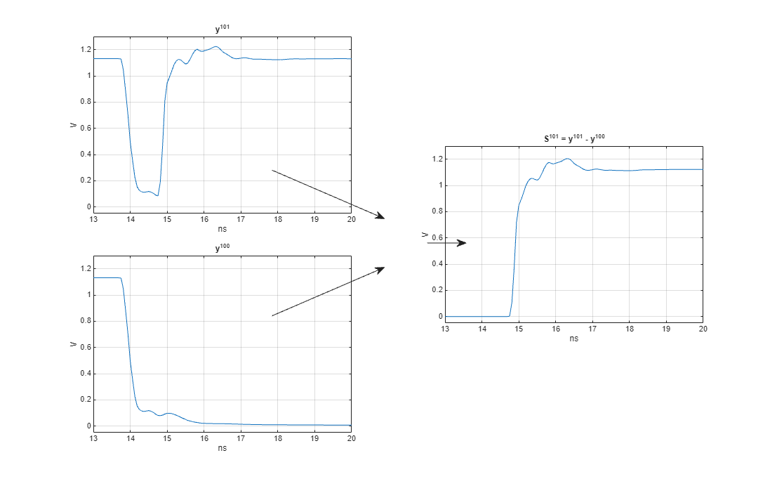
Take a closer look at the calculation . By subtracting from , remove the effect of the prior symbol pattern, 10, from the edge response. This process effectively conditions the step response on the preceding 10 symbol pattern.
% Create time vector
t = RepresentationMER2.SampleInterval*(0:size(RepresentationMER2.SourceWaves,1)-1);

% Create illustration of how the effective step response is calculated
h8 = figure('IntegerHandle','off');
tiledlayout(4,2)
ax7(1) = nexttile(1,[2 1]);
plot(t*1e9,RepresentationMER2.SourceWaves(:,6)),
title(RepresentationMER2.SourceWaveLabel(6))
ylabel('V'),xlabel('ns'),grid on
ax7(2) = nexttile(5,[2 1]);
plot(t*1e9,RepresentationMER2.SourceWaves(:,5)),
title(RepresentationMER2.SourceWaveLabel(5))
ylabel('V'),xlabel('ns'),grid on
ax7(3) = nexttile(4,[2 1]);
plot(t*1e9,RepresentationMER2.EffectiveSteps(:,3)),
title(sprintf('%s = %s - %s',RepresentationMER2.EffectiveStepsLabel{3},RepresentationMER2.SourceWaveLabel{6},RepresentationMER2.SourceWaveLabel{5}))
ylabel('V'),xlabel('ns'),grid on

linkaxes(ax7,'xy')
xlim([13 20])
ylim([-0.05 1.3])

set(h8,'Units','normalized','Position',[ 0 0 1 1]);

% Draw arrows
annotation('textarrow',[0.35 0.495],[0.65 0.55])
annotation('textarrow',[0.35 0.495],[0.35 0.45])
annotation('textarrow',[0.55 0.6],[0.5 0.5])
Note that for NRZ, the number of required waveforms doubles with each increase in MER order. Also, if the circuit simulator is perfectly time-invariant, you can obtain the source waveform by simply delaying the waveform, rather than running a separate simulation. Similar manipulations can help reduce the circuit simulation workload when you explore higher-order MER analysis.
Appendix B: Step Response Self-Consistency
Numerical uncertainty affects any computational analysis, but it becomes especially noticeable when multiple system measurements show slight inconsistencies. For example, a discretely sampled impulse response is self-consistent if it starts and ends at 0 Volts. Although this condition is rarely met exactly, it is usually close enough that the resulting numerical uncertainty is insignificant and can be ignored.
Similarly, when using circuit-simulated step responses for MER system characterization, the initial symbol voltage of the falling step response rarely matches the terminal voltage of the rising step response. More importantly, the voltage swing between the initial and terminal values usually differs between the rising and falling edge responses. These inconsistencies can accumulate during MER waveform generation and statistical analysis, introducing unwanted artifacts into the results.
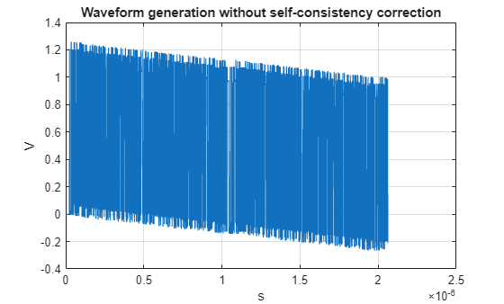
To illustrate the impact of the mismatch between the rising edge voltage swing and the falling edge voltage swing, disable the self consistency correction and generate a long PRBS waveform which will display a voltage drift.
ApplyStepSelfConsistency = false;

% Create MER object
RepresentationMER1uncorrected = si.MER(...
    'Order', 1,...
    'Modulation', 2,...
    'SamplesPerSymbol', SamplesPerSymbol,...
    'PlotAxis', 'Seconds',...
    'SymbolTime', simDataOrder1.SymbolTime,...
    'Specification', 'Wave',...
    'SourceWaves', simDataOrder1.PatternWave,...
    'SourceWavesPattern', simDataOrder1.PatternMat,...
    'ApplyStepSelfConsistency',ApplyStepSelfConsistency,...
    'ReferenceWave',simDataOrder1.ReferenceWave,...
    'ReferenceWavePattern',simDataOrder1.ReferencePattern);

% Generate waveform
wave = makeWave(RepresentationMER1uncorrected,prbs(11,2^11-1));
t2 = RepresentationMER1uncorrected.SampleInterval*(0:length(wave)-1);

% Visualize waveform
h9 = figure('IntegerHandle','off');
plot(t2,wave)
xlabel('s')
ylabel('V')
title('Waveform generation without self-consistency correction')
grid on
For the MER order 1 source waveforms, the following table presents the initial voltage, terminal voltage, voltage swing (the difference between initial and terminal voltages) and the differences in voltage swing.
InitialVoltage = RepresentationMER1uncorrected.SourceWaves(1,:)';
TerminalVoltage = RepresentationMER1uncorrected.SourceWaves(end,:)';
VoltageSwing = TerminalVoltage - InitialVoltage;
AverageSwing = mean(abs(VoltageSwing(2:3)));
SwingError = [NaN; AverageSwing - abs(VoltageSwing(2:3));NaN];
disp(table(InitialVoltage,TerminalVoltage,VoltageSwing,SwingError,...
'RowNames',RepresentationMER1uncorrected.SourceWaveLabel));
              InitialVoltage    TerminalVoltage    VoltageSwing    SwingError
              ______________    _______________    ____________    ___________

    y^{00}             0                  0                0               NaN
    y^{01}             0             1.1294           1.1294        0.00026149
    y^{10}        1.1311           0.001155            -1.13       -0.00026149
    y^{11}        1.1311             1.1311                0               NaN
The swing error is also returned by the MER object itself:
disp(RepresentationMER1.TerminalError)
   1.0e-03 *

    0.2615   -0.2615
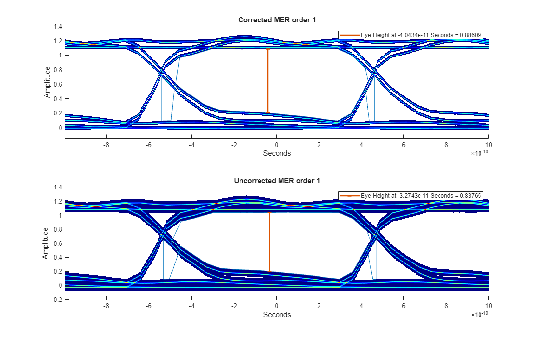
For the MER representation to be self consistent, the voltage swing of all the effective step responses needs to be identical. The correction is done by first calculating the average swing voltage of all the effective step responses, then scaling each effective step response to guarantee this swing. The impact of this correction on the MER order 1 statistical eyes is shown below.
h10 = figure('IntegerHandle','off');
nexttile
eyeCenterTime=RepresentationMER1.StatEyeInfo.EyeObj.eyeCenter;
RepresentationMER1.StatEyeInfo.EyeObj.eyeHeight(eyeCenterTime,'Plot','on');
title('Corrected MER order 1')
colorbar off

nexttile

eyeCenterTime=RepresentationMER1uncorrected.StatEyeInfo.EyeObj.eyeCenter;
RepresentationMER1uncorrected.StatEyeInfo.EyeObj.eyeHeight(eyeCenterTime,'Plot','on');
colorbar off
title('Uncorrected MER order 1')
set(h10,'Units','normalized','Position',[ 0 0 1 1]);
For MER order 2, there are four effective step responses, each of which can have their own unique voltage swing. The voltage swing error in Volts is reported as follows:
disp(RepresentationMER2.TerminalError)
   1.0e-03 *

    0.2615    0.2597   -0.2598   -0.2614
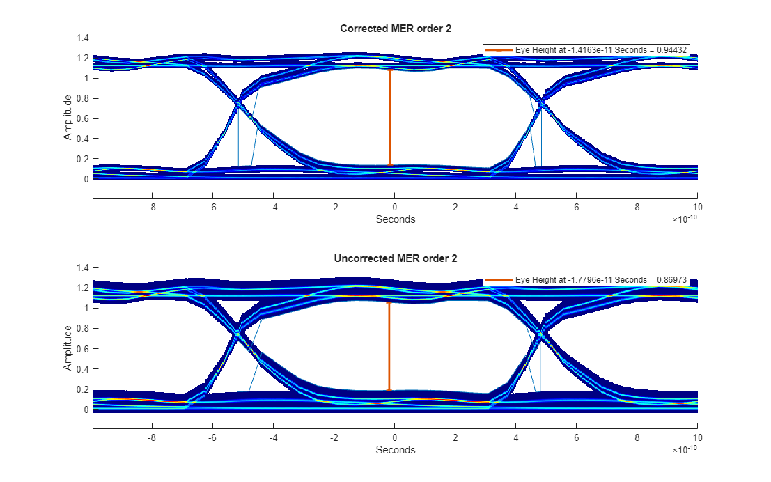
The impact of the voltage swing variation on the eye diagram is shown below for MER order 2.
ApplyStepSelfConsistency = false;

% Create MER object
RepresentationMER2uncorrected = si.MER(...
    'Order', 2,...
    'Modulation', 2,...
    'SamplesPerSymbol', SamplesPerSymbol,...
    'PlotAxis', 'Seconds',...
    'SymbolTime', simDataOrder2.SymbolTime,...
    'Specification', 'Wave',...
    'SourceWaves', simDataOrder2.PatternWave,...
    'SourceWavesPattern', simDataOrder2.PatternMat,...
    'ApplyStepSelfConsistency',ApplyStepSelfConsistency,...
    'ReferenceWave',simDataOrder2.ReferenceWave,...
    'ReferenceWavePattern',simDataOrder2.ReferencePattern);

h11 = figure('IntegerHandle','off');clf
nexttile
eyeCenterTime=RepresentationMER2.StatEyeInfo.EyeObj.eyeCenter;
RepresentationMER2.StatEyeInfo.EyeObj.eyeHeight(eyeCenterTime,'Plot','on');
title('Corrected MER order 2')
colorbar off

nexttile

[eyeCenterTime]=RepresentationMER2uncorrected.StatEyeInfo.EyeObj.eyeCenter;
RepresentationMER2uncorrected.StatEyeInfo.EyeObj.eyeHeight(eyeCenterTime,'Plot','on');
colorbar off
title('Uncorrected MER order 2')
set(h11,'Units','normalized','Position',[ 0 0 1 1]);
The value of the step response self-consistency enforcement is found when comparing the plotValidation results for the two cases. The time domain waveform generation for unmodified case will slowly creep up (or down) depending on the voltage swing error.
The step response self-consistency modification is only enabled for NRZ signals. The MATLAB si.MER object class can perform PAMn waveform generation and statistical eye analysis when provided with the necessary inputs but at this time the self correction is for NRZ only.
References
[1] Lambrecht, Frank, Ching-Chao Huang, and Michael Fox. Technique for determining performance characteristics of electronic systems. United States Patent US6775809B1.
[2] Ren, JiHong, and Kyung Suk Oh. Multiple Edge Responses for Fast and Accurate System Simulations. IEEE Transactions on Advanced Packaging 31, no. 4 (2008): 741–48. https://doi.org/10.1109/TADVP.2008.2002201.
[3] Chou, Chiu-Chih, Sheng-Yun Hsu, and Tzong-Lin Wu. Estimation Method for Statistical Eye Diagram in a Nonlinear Digital Channel. IEEE Transactions on Electromagnetic Compatibility 57, no. 6 (2015): 1655–64. https://doi.org/10.1109/TEMC.2015.2457928.