Stability Analysis Using Disk Margins
Disk margins quantify the stability of a closed-loop system against gain or phase variations in the open-loop response. In disk-based margin calculations, the software models such variations as disk-shaped multiplicative uncertainty on the open-loop transfer function. The disk margin measures how much uncertainty the loop can tolerate before going unstable.
That uncertainty amount corresponds to minimum gain and phase margins. The disk-based gain margin DGM is the amount by which the loop gain can increase or decrease without loss of stability, in absolute units. The disk-based phase margin DPM is the amount by which the loop phase can increase or decrease without loss of stability, in degrees. These disk-based margins take into account all frequencies and loop interactions. Therefore, disk-based margin analysis provides a stronger guarantee of stability than the classical gain and phase margins.
Robust Control Toolbox™ provides tools to:
Analyze system stability against gain and phase variations. Use
diskmarginto compute the disk-based gain and phase margins of SISO and MIMO feedback loops.Model gain and phase uncertainty. Use the
umargincontrol design block to analyze the effect of gain and uncertainty on system performance and stability.
Modeling Gain and Phase Variations
Both umargin and diskmargin represent gain and phase variation as a multiplicative complex factor F(s), replacing the nominal open-loop response L(s) with L(s)*F(s). The factor F takes values in a disk that includes the nominal value F = 1. This multiplicative factor models both gain and phase variations. For instance, the following plot shows one such disk in the complex plane.
DGM = [0.6,1.7];
diskmarginplot(DGM,'disk')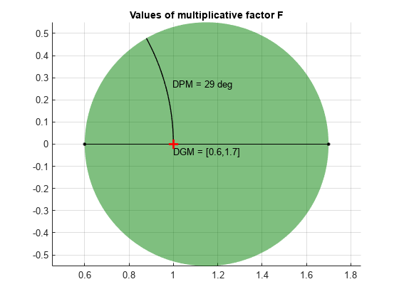
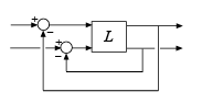
The values in this disk encompass relative gain-only variations in the range DGM = [0.6,1.7], or ±4 dB. They also represent absolute phase-only variations of DPM = [–29,29], or ±29°. Consider the following closed-loop system, with nominal loop transfer L and unit feedback.
If this feedback loop remains stable for all values of F in the disk shown in the previous plot, then the disk-based gain margin of L is at least DGM, and the disk-based phase margin is at least DPM.
Both umargin and diskmargin model gain and phase uncertainty with a family of disks described by two parameters, α and σ. For SISO systems, the disk is parameterized by:
In this model,
δ is the normalized uncertainty (an arbitrary complex value in the unit disk |δ| < 1).
α sets the amount of gain and phase variation modeled by F. For fixed σ, the parameter α controls the size of the disk. For α = 0, the multiplicative factor is 1, corresponding to the nominal L.
σ, called the skew, biases the modeled uncertainty toward gain increase or gain decrease.
Each α,σ pair corresponds to a disk that models a particular gain-variation range DGM = [gmin,gmax], given by the points where the disk intercepts the real (x) axis. The corresponding phase variation DPM is determined by the angle between the real axis and a line through the origin and tangent to the disk. Thus you can describe a modeled set of gain and phase variations entirely by either the two values α,σ or the two values DGM = [gmin,gmax]. σ = 0 models a balanced gain variation with [gmin,gmax] such that gmin = 1/gmax. When σ < 0, then F represents a larger gain decrease than increase (gmin < 1/gmax). Conversely σ > 0 represents a larger gain increase than decrease. For instance, consider the disks parameterized by α = 0.5 and three different skews, σ = –2, 0, and 2.
diskmarginplot(0.5,[-2 0 2],'disk')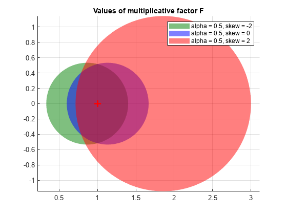
Each α,σ pair corresponds to a disk that models a different gain-variation range DGM = [gmin,gmax]. Examine the gain variations that correspond to each of these three disks.
Ranges = dm2gm(0.5,[-2 0 2])
Ranges = 3×2

    0.3333    1.4000
    0.6000    1.6667
    0.7143    3.0000
diskmarginplot(Ranges)
The balanced σ = 0 range is symmetric around the nominal value, allowing the gain to increase or decrease by a factor of about 1.67. The negative σ value corresponds to more gain decrease than increase, while positive σ gives more increase than decrease.
The umargin control design block uses this model to represent gain and phase uncertainty in a feedback loop, setting α and σ from the gain and phase margin values you specify when you create the block. The diskmargin command uses this model to compute disk-based gain and phase margins as discussed in the next section.
Disk Margins for SISO Loops
For a loop transfer L and a given skew σ, the diskmargin command finds the largest disk size α at which the closed-loop system feedback(L*F,1) is stable for all values of F. This value of α is called the disk margin. The disk-based gain margin DGM and disk-based phase margin DPM are the range of gain and phase variations represented by the corresponding disk.
For instance, compute the disk margin and associated disk-based gain and phase margins for a SISO transfer function, using the default σ = 0.
sigma = 0;
L = tf(25,[1 10 10 10]);
DM = diskmargin(L,sigma);
alpha = DM.DiskMargin
alpha =
0.4581
DGM = DM.GainMargin
DGM = 1×2

    0.6273    1.5942
DPM = DM.PhaseMargin
DPM = 1×2

  -25.8017   25.8017
For this system, the balanced (σ = 0) disk margin α is about 0.46. The corresponding disk-based gain margin DGM shows that the system remains stable for relative variations in gain between about 0.63 and 1.6, or for phase variations of about ±26 degrees. This result establishes stability for all values of F of in the disk:
diskmarginplot(DGM,'disk')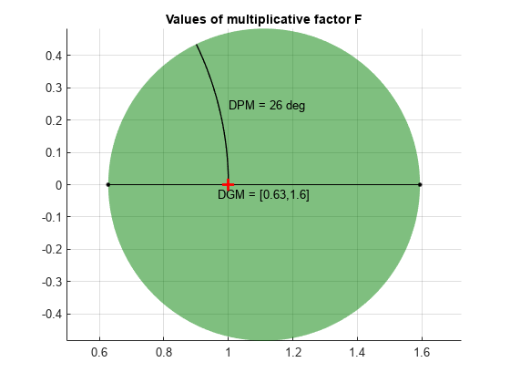
The gain margins are the intersection of the disk with the real axis. The phase margin is the largest angle between the real axis and a line through the origin tangent to the disk.
Combined Gain and Phase Variations
The gain margins DGM you obtain from diskmargin assume no phase variation, and the phase margins DPM assume no gain variation. In practice, your system can experience simultaneous gain and phase variations. diskmarginplot lets you visualize the ranges of simultaneous gain and phase variations that the system can tolerate.
diskmarginplot(DGM)
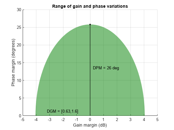
The shaded region shows the stable range of combined gain and phase variations. Thus, for instance, with no phase variation, the system can tolerate the full range DGM of gain variation, about –4 dB to 4 dB. If the phase is allowed to vary by ±17 degrees or so, the allowable gain variation drops to a range of about –3 dB to 3 dB.
Disk Margins and Skew
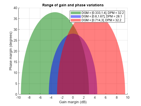
The ranges shown above, computed for σ = 0, represent a balanced gain variation, where gmin = 1/gmax. Varying the skew can reveal whether the loop is more sensitive to gain increase or decrease. For example, using σ > 0 may reveal that the feedback loop is very robust to gain increase, because positive σ models more gain increase than decrease. This result, however, says little about robustness to gain decrease. Try computing the disk-based gain and phase margins for L, biasing the margins toward gain increase or gain decrease.
DMdec = diskmargin(L,-2);
DMinc = diskmargin(L,2);
DGMdec = DMdec.GainMargin
DGMdec = 1×2

    0.4013    1.3745
DGMinc = DMinc.GainMargin
DGMinc = 1×2

    0.7717    1.7247
Put together, these results show that in the absence of phase variation, stability is maintained for relative gain variations between 0.4 and 1.72. To see how the phase margin depends on these gain variations, plot the stable ranges of gain and phase variations for each diskmargin result.
diskmarginplot([DGMdec;DGM;DGMinc])
legend('\sigma = -2','\sigma = 0','\sigma = 2')
title('Stable range of gain and phase variations')
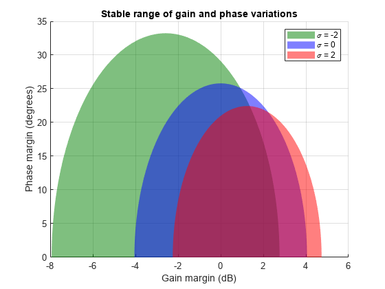
This plot shows that the feedback loop can tolerate larger phase variations when the gain decreases. In other words, the loop stability is more sensitive to gain increase. Note that it would be misleading to just take the largest reported phase margin (nearly 30 degrees for σ = –2). Indeed, this large value is predicated on a small gain increase of less than 3 dB. Since both gain and phase are subject to uncertainty in general, it is important to pay attention to combined variations. For example, the plot shows that when the gain increases by 4 dB, the phase margin drops to less than 15 degrees. By contrast, it remains greater than 30 degrees when the gain decreases by 4 dB.
In conclusion, varying the skew σ can give a fuller picture of sensitivity to gain and phase uncertainty. Unless you are mostly concerned with gain variations in one direction (increase or decrease), it is not recommended to draw conclusions from a single nonzero value of σ. Instead use the default σ = 0 to get unbiased estimates of gain and phase margins. When using nonzero values of σ, use both positive and negative values to compare relative sensitivity to gain increase vs. gain decrease.
Uncertainty Disk in the Nyquist Plane
The requirement of robust stability for the closed-loop system feedback(L*F,1) is equivalent to a requirement that 1 + L*F ≠ 0. In the Nyquist plane, this requirement becomes L(jω) ≠ –1/F. Thus the disk F for each value of σ defines an exclusion region that the Nyquist curve does not enter if closed-loop stability is preserved. All such disks –1/F contain the critical point (–1,0) and are tangent to the Nyquist curve. The skew adjusts the size and position of the tangent disks, as illustrated in the following plot, which shows the exclusion regions for the three disk margins of L computed above. As σ increases, each disk provides lower estimates of the classical gain and phase margins.
figure
h = nyquistplot(L);
hold on
diskmarginplot([DGMdec;DGM;DGMinc],'nyquist')
h.Responses(2).Name = '\sigma = -2';
h.Responses(3).Name = '\sigma = 0';
h.Responses(4).Name = '\sigma = 2';
hold off
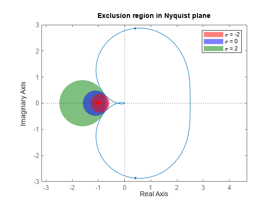
For more details about the Nyquist interpretation of the uncertainty disk, see Disk Margin and Smallest Destabilizing Perturbation.
MIMO Uncertainty Model and Disk Margins of MIMO Feedback Loops
For MIMO systems, the model applies an independent uncertainty disk Fj to each loop channel, given by
The model replaces the MIMO open-loop response L with L*F, where
Analogous to the SISO case, the disk margin is the largest value of
α for which the closed-loop system
feedback(L*F,eye(N)) is stable for all values of
F. It can be useful to consider independent variations across
all feedback channels at once, as well as variations in individual channels.
Therefore, diskmargin lets you compute:
Loop-at-a-time margins — Maximum tolerable gain variations (or phase variations) in each feedback channel, computed with all other loops closed. Loop-at-a-time analysis effectively sets all δj to 0 for all channels except the channel under analysis.
Multiloop margins — Maximum tolerable gain variations (or phase variations) across all feedback channels. Multiloop margins allow for independent variations in all feedback channels at the same time. The ability to capture such loop interactions is a key advantage of the disk-margin approach over classical margin analysis. Multiloop analysis typically yield smaller margins than loop-at-a-time analysis.
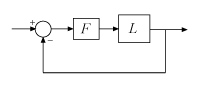
For instance, consider the 2-channel MIMO system of the following illustration.
For this system, you can compute:
Maximum tolerable gain variations (or phase variations) in the first channel (first system input to first system output)
Maximum tolerable gain variations (or phase variations) in the second channel (second system input to second system output)
Maximum tolerable independent gain variations (or phase variations) in both channels at the same time.
For details and examples of how to get these loop-at-a-time and multiloop margins,
see diskmargin.
Variations at Plant Input or Plant Output
In some cases, the stability margins can vary depending on whether gain and phase
variations are applied at the plant input or the plant output.
diskmargin lets you compute margins for variations at the
input, output, or both simultaneously. In general, the margins for simultaneous
input and output variations are smaller than those for input or output only, and
provide a more conservative guarantee of stability. Consider the SISO or MIMO
closed-loop system of the following diagram.
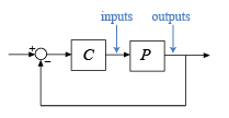
You can compute the disk margins at the plant inputs and outputs as follows.
[DM,MM] = diskmargin(P*C)returns the margins for variations at the plant outputs.[DM,MM] = diskmargin(C*P)returns the margins for variations at the plant inputs.MMIO = diskmargin(P,C)returns the margin for simultaneous variations at the plant outputs and inputs. When comparing this margin to the margins at either the inputs or outputs, use2*MMIO.Diskmargin, to account for the simultaneous perturbations applied at both inputs and outputs.
Frequency Dependence of Margins
In general, gain and phase margins vary across frequency. This variation is due to the frequency variation of the open-loop response L: For each frequency ω, there is a different largest α(ω) such that I + L(jω)F is invertible for all values of F in the disk. This value is the first α(ω) for which the closed-loop pole crosses the jω axis at the frequency ω, becoming unstable.
As the disk margin α varies across frequency, so does the corresponding tolerable range of gain or phase variations. Plotting these disk-based margins as a function of frequency provides information about frequency bands with weak margins.
L = tf(25,[1 10 10 10]);
diskmarginplot(L)
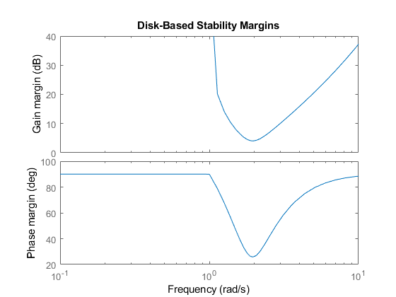
The disk margins returned by diskmargin are the minimum such
values over all frequencies. Right-click on the plot generated by
diskmarginplot for a data tip with information about these
values.
Worst-Case Disk Margins
The disk margin is computed by applying an uncertainty to the nominal loop transfer L and computing how large that uncertainty can be while preserving closed-loop stability. If the loop transfer L is itself an uncertain system, then the disk margin also varies as a function of the other uncertainties in the system. The worst-case disk margin is the smallest disk margin that occurs within the ranges of the uncertainties modeled in L. It is also the minimum guaranteed margin over the uncertainty range.
Compute worst-case disk margins of an uncertain system using wcdiskmargin. This function estimates the worst-case disk margins
and corresponding worst-case gain and phase margins for both loop-at-a-time and
multiloop variations. The function also returns the worst-case perturbation, the
combination of uncertain elements in L that yields the weakest
margins. You can visualize worst-case disk-based margins with wcdiskmarginplot.
Disk Margins and Control System Tuning
Tuning with systune or Control System Tuner
The control system tuning tools in Control System Toolbox™ let you specify target gain and phase margins for loops in your
tuned system. The tuning goals TuningGoal.Margins (for
command-line tuning with systune) and Margins Goal (for
tuning with Control System Tuner) use disk-based margins. Thus, when you specify
independent gain and phase margins GM and
PM for tuning, the software chooses the smallest
α that enforces both values. This α is
given by:
In applying this value of α, the tuning software assumes σ = 0.
Visualizing margin goals using viewGoal or Control System
Tuner tuning-goal plots is equivalent to diskmarginplot(L),
where L is the tuned open-loop response.
Robust Design with musyn
When you perform robust controller tuning with musyn, you
can model gain and phase variations directly in your system using
umargin. Then, performing robust controller design with
musyn enforces robust stability for the modeled range
of gain and phase variations. This approach is useful because it allows you to
study the effects of the expected gain and phase variations on all aspects of
system performance using the same model you use for tuning. For an example, see
Robust Controller for Spinning Satellite.
A disadvantage of this approach is that musyn does not
only enforce robust stability over the entire modeled uncertainty range. It also
attempts to enforce robust performance. (See Robust Performance Measure for Mu Synthesis.) Achieving
this more stringent requirement is typically impossible or results in
intolerable degradation of nominal performance. Thus, you might need to reduce
the modeled gain and phase variations to maintain reasonable performance.
systune and Control System Tuner do not have this
drawback because they handle margin goals independently of any performance
goals.
More About Disk Margins
For more information about disk margins, play the video.
References
[1] Blight, James D., R. Lane Dailey, and Dagfinn Gangsaas. “Practical Control Law Design for Aircraft Using Multivariable Techniques.” International Journal of Control 59, no. 1 (January 1994): 93–137. https://doi.org/10.1080/00207179408923071.
[2] Seiler, Peter, Andrew Packard, and Pascal Gahinet. “An Introduction to Disk Margins [Lecture Notes].” IEEE Control Systems Magazine 40, no. 5 (October 2020): 78–95.
See Also
diskmargin | wcdiskmargin | diskmarginplot | umargin