MIMO Stability Margins for Spinning Satellite
This example shows that in MIMO feedback loops, disk margins are more reliable stability margin estimates than the classical, loop-at-a-time gain and phase margins. It first appeared in Reference [1].
Spinning Satellite
This example is motivated by controlling the transversal angular rates in a spinning satellite (see Reference [2]). The cylindrical body spins around its axis of symmetry ( axis) with constant angular rate . The goal is to independently control the angular rates and around the and axes using torques and . The equations of motion lead to the second-order, two-input, two-output model:
Consider a static control law that combines feedforward and unit-feedback actions:
.
Setting the feedforward gain as follows achieves perfect decoupling and makes each loop respond as a first-order system with unit time constant.
The resulting system is the two-loop control system of the following diagram.
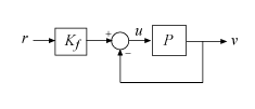
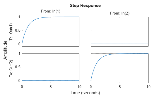
Create a state-space model of the satellite and the controller to see the performance of the system with this controller.
% Plant
a = 10;
A = [0 a;-a 0];
B = eye(2);
C = [1 a;-a 1];
D = 0;
P = ss(A,B,C,D);

% Prefilter
Kf = [1 -a;a 1]/(1+a^2);

% Closed-loop model
T = feedback(P,eye(2))*Kf;
step(T,10)
Loop-at-a-Time Gain and Phase Margins
The classical gain and phase margins are a customary way to gauge the robustness of SISO feedback loops to plant uncertainty. In MIMO control systems, the gain and phase margins are often assessed one loop at a time, meaning that the margins are computed independently for each feedback channel with the other loops closed. Robustness is clearly in doubt when one loop is found to have weak margins. Unfortunately, the converse is not true. Each individual loop can have strong gain and phase margins while overall robustness is weak. This is because the loop-at-a-time approach fails to account for loop interactions and conditioning of the MIMO loop transfer. The spinning satellite example is a perfect illustration of this point.
To compute the loop-at-a-time gain and phase margins, introduce an analysis point at the plant input to facilitate access to the open-loop responses.
uAP = AnalysisPoint('u',2);
T = feedback(P*uAP,eye(2))*Kf;
Use getLoopTransfer to access the SISO loop transfers at with the loop closed, and at with the loop closed.
Lx = getLoopTransfer(T,'u(1)',-1);
Ly = getLoopTransfer(T,'u(2)',-1);
Finally, use margin to compute the loop-at-a-time classical gain and phase margins.
[gmx,pmx] = margin(Lx)
gmx =
Inf
pmx =
90
[gmy,pmy] = margin(Ly)
gmy =
Inf
pmy =
90
margin reports a gain margin of Inf and phase margin of 90°, as stable against variations in gain and phase as a SISO loop can be. This result is not surprising given that the loop transfers Lx and Ly are pure integrators.
tf(Lx), tf(Ly)
ans =

  From input "u(1)" to output "u(1)":
  1
  -
  s

Continuous-time transfer function.
Model Properties

ans =

  From input "u(2)" to output "u(2)":
  1
  -
  s

Continuous-time transfer function.
Model Properties
Despite this loop-at-a-time result, the MIMO feedback loop T can be destabilized by a 10% gain change affecting both loops. To demonstrate this destabilization, multiply the plant by a static gain that decreases the gain by 10% in the channel and increases it by 10% in the channel. Then compute the poles of the unit feedback loop to see that one of them has moved into the right half-plane, driving the loop unstable.
dg = diag([1-0.1,1+0.1]);
pole(feedback(P*dg,eye(2)))
ans = 2×1

   -2.0050
    0.0050
Because model uncertainty typically affects all feedback loops, the loop-at-a-time margins tend to overestimate actual robustness and can miss important issues with MIMO designs.
Disk Margins
The notion of disk margin gives a more comprehensive assessment of robustness in MIMO feedback loops by explicitly modeling and accounting for loop interactions. See Stability Analysis Using Disk Margins for additional background information. To compute the SISO and MIMO disk margins for the spinning satellite example, extract the MIMO loop transfer L and use the diskmargin command.
L = getLoopTransfer(T,'u',-1);
[DM,MM] = diskmargin(L);
The first output DM contains the loop-at-a-time disk-based margins. These are lower estimates of the classical gain and phase margins. For this model, the disk-based margins also report a gain margin of Inf and phase margin of 90° for each individual loop. So far nothing new.
DM(1)
ans = struct with fields:
           GainMargin: [0 Inf]
          PhaseMargin: [-90 90]
           DiskMargin: 2
           LowerBound: 2
           UpperBound: 2
            Frequency: 0
    WorstPerturbation: [2×2 ss]
DM(2)
ans = struct with fields:
           GainMargin: [0 Inf]
          PhaseMargin: [-90 90]
           DiskMargin: 2
           LowerBound: 2
           UpperBound: 2
            Frequency: 0
    WorstPerturbation: [2×2 ss]
The second output MM contains the MIMO disk-based margins.
MM
MM = struct with fields:
           GainMargin: [0.9051 1.1049]
          PhaseMargin: [-5.7060 5.7060]
           DiskMargin: 0.0997
           LowerBound: 0.0997
           UpperBound: 0.0999
            Frequency: 1.0000e-04
    WorstPerturbation: [2×2 ss]
This multiloop disk-based margin is the most reliable measure of MIMO robustness since it accounts for independent gain and phase variations in all loop channels at the same time. Here MM reports a gain margin of [0.905,1.105], meaning that the open-loop gain can increase or decrease by a factor of 1.105 while preserving closed-loop stability. The phase margin is 5.7°. This result is in line with the destabilizing perturbation dg above which corresponds to a relative gain change in the range [0.90,1.10].
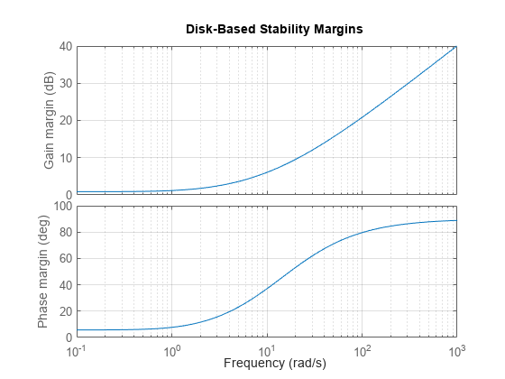
The diskmarginplot command lets you visualize the disk-based margins as a function of frequency. For this system, that the disk-based margins are weakest near DC (zero frequency).
clf
diskmarginplot(L)
grid
The struct MM also contains the smallest destabilizing perturbation MM.WorstPerturbation. This dynamic perturbation is a realization of the smallest destabilizing change in gain and phase. Note that this perturbation modifies both gain and phase in both feedback channels.
WGP = MM.WorstPerturbation;
pole(feedback(P*WGP,eye(2)))
ans = 8×1 complex

  -1.0000 + 0.0001i
  -1.0000 - 0.0001i
  -0.0002 + 0.0002i
  -0.0002 - 0.0002i
   0.0000 + 0.0001i
   0.0000 - 0.0001i
  -0.0000 + 0.0000i
  -0.0000 - 0.0000i
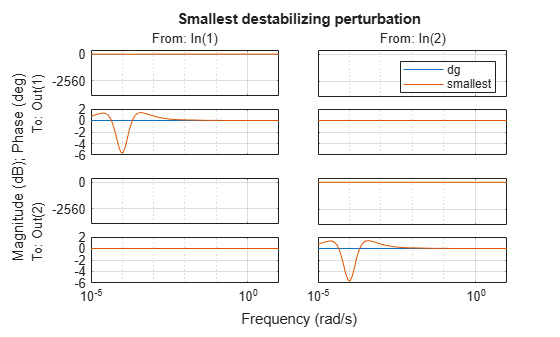
Compare the dynamic perturbation WGP with the static gain dg used above to destabilize the system.
bode(ss(dg),WGP), grid
title('Smallest destabilizing perturbation')
legend('dg','smallest')
Conclusion
For multi-loop control systems, disk margins are a more reliable robust stability test than loop-at-a-time gain and phase margins. The diskmargin function computes both loop-at-a-time and MIMO disk margins and the corresponding smallest destabilizing perturbations. You can use these perturbations for further analysis and risk assessment, for example, by injecting them in a detailed nonlinear simulation of the system.
To learn how to design a controller with adequate stability margins for this plant, see the example Robust Controller for Spinning Satellite.
References
[1] Doyle, J. “Robustness of Multiloop Linear Feedback Systems.” In 1978 IEEE Conference on Decision and Control Including the 17th Symposium on Adaptive Processes, 12–18. San Diego, CA, USA: IEEE, 1978. https://doi.org/10.1109/CDC.1978.267885.
[2] Zhou, K., J.C.Doyle, and K. Glover. Robust and Optimal Control, Englewood Cliffs, NJ: Prentice-Hall, 1996, Section 9.6.