fitmagfrd
Fit frequency response magnitude data with minimum-phase state-space model using log-Chebyshev magnitude design
Description
Examples
Create frequency response magnitude data from a fifth-order system.
sys = tf([1 2 2],[1 2.5 1.5])*tf(1,[1 0.1]);
sys = sys*tf([1 3.75 3.5],[1 2.5 13]);
omega = logspace(-1,1);
sysg = abs(frd(sys,omega));
bodemag(sysg,'r');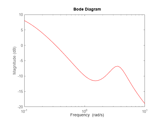
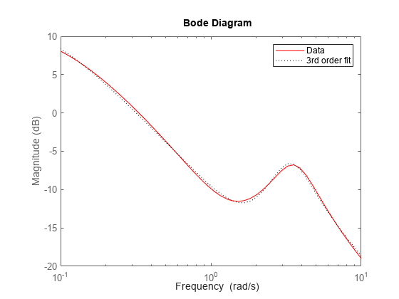
Fit the magnitude data with a minimum-phase, stable third-order system.
ord = 3;
b1 = fitmagfrd(sysg,ord);
b1g = frd(b1,omega);
bodemag(sysg,'r',b1g,'k:');
legend('Data','3rd order fit');
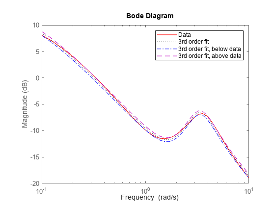
Fit the magnitude data with a third-order system constrained to lie below and above the given data.
C2.UpperBound = sysg;
C2.LowerBound = [];
b2 = fitmagfrd(sysg,ord,[],[],C2);
b2g = frd(b2,omega);
C3.UpperBound = [];
C3.LowerBound = sysg;
b3 = fitmagfrd(sysg,ord,[],[],C3);
b3g = frd(b3,omega);
bodemag(sysg,'r',b1g,'k:',b2g,'b-.',b3g,'m--')
legend('Data','3rd order fit','3rd order fit, below data',...
       '3rd order fit, above data')
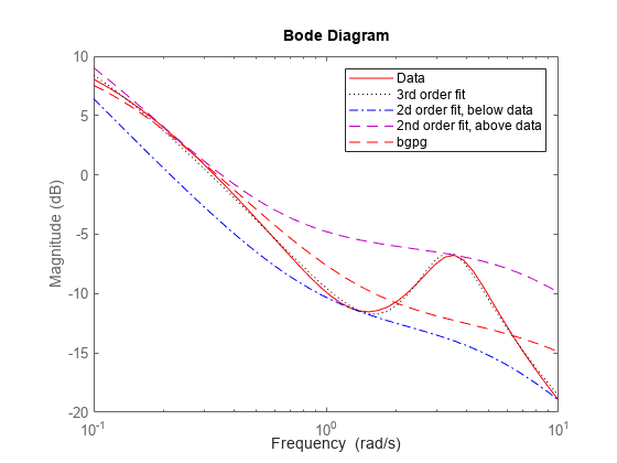
Fit the magnitude data with a second-order system constrained to lie below and above the given data.
ord = 2;
C2.UpperBound = sysg;
C2.LowerBound = [];
b2 = fitmagfrd(sysg,ord,[],sysg,C2);
b2g = frd(b2,omega);
C3.UpperBound = [];
C3.LowerBound = sysg;
b3 = fitmagfrd(sysg,ord,[],sysg,C3);
b3g = frd(b3,omega);
bgp = fitfrd(genphase(sysg),ord);
bgpg = frd(bgp,omega);
bodemag(sysg,'r',b1g,'k:',b2g,'b-.',b3g,'m--',bgpg,'r--')
legend('Data','3rd order fit','2d order fit, below data',...
       '2nd order fit, above data','bgpg')
Input Arguments
Output Arguments
Algorithms
fitmagfrd uses a version of log-Chebyshev magnitude design,
solving
   min f     subject to (at every frequency point in A):
           |d|^2 /(1+ f/WT) < |n|^2/A^2 < |d|^2*(1 + f/WT)
plus additional constraints imposed with C. Here n
and ddenote the numerator and denominator, respectively, and B =
n/d. n and d have orders
(N-RD) and N, respectively. The problem is solved
using linear programming for fixed f and bisection to minimize
f. An alternate approximate method, which cannot enforce the constraints
defined by C, is B =
fitfrd(genphase(A),N,RD,WT).
References
[1] Oppenheim, A.V., and R.W. Schaffer, Digital Signal Processing, Prentice Hall, New Jersey, 1975, p. 513.
[2] Boyd, S. and Vandenberghe, L., Convex Optimization, Cambridge University Press, 2004.
Version History
Introduced before R2006a