Robust Tuning of DC Motor Controller
This example shows how to robustly tune a PID controller for a DC motor with imperfectly known parameters.
DC Motor Modeling
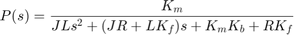
An uncertain model of the DC motor is derived in the "Robustness of Servo Controller for DC Motor" example. The transfer function from applied voltage to angular velocity is given by
where the resistance  , the inductance
  , the EMF constant
  , armature constant
  , viscous friction
  , and inertial load
  are physical parameters of the motor. These parameters are not perfectly known and are subject to variation, so we model them as uncertain values with a specified range or percent uncertainty.
R = ureal('R',2,'Percentage',40);
L = ureal('L',0.5,'Percentage',40);
K = ureal('K',0.015,'Range',[0.012 0.019]);
Km = K; Kb = K;
Kf = ureal('Kf',0.2,'Percentage',50);
J = ureal('J',0.02,'Percentage',20);

P = tf(Km,[J*L J*R+Kf*L Km*Kb+Kf*R]);
P.InputName = 'Voltage';
P.OutputName = 'Speed';
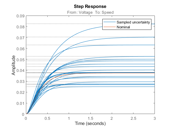
Time and frequency response functions like step or bode automatically sample the uncertain parameters within their range. This is helpful to gauge the impact of uncertainty. For example, plot the step response of the uncertain plant P and note the large variation in plant DC gain.
step(P,getNominal(P),3)
legend('Sampled uncertainty','Nominal')
Robust PID Tuning
To robustly tune a PID controller for this DC motor, create a tunable PID block C and construct a closed-loop model CL0 of the feedback loop in Figure 1. Add an analysis point dLoad at the plant output to measure the sensitivity to load disturbance.
C = tunablePID('C','pid');
AP = AnalysisPoint('dLoad');
CL0 = feedback(AP*P*C,1);
CL0.InputName = 'SpeedRef';
CL0.OutputName = 'Speed';
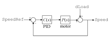
Figure 1: PID control of DC motor
There are many ways to specify the desired performance. Here we focus on sensitivity to load disturbance, roll-off, and closed-loop dynamics.
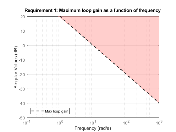
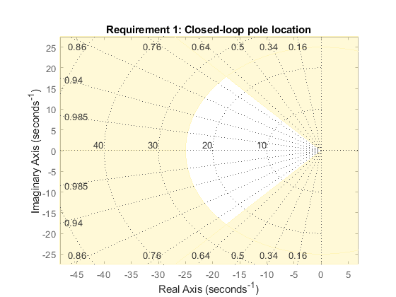
R1 = TuningGoal.Sensitivity('dLoad',tf([1.25 0],[1 2]));
R2 = TuningGoal.MaxLoopGain('dLoad',10,1);
R3 = TuningGoal.Poles('dLoad',0.1,0.7,25);
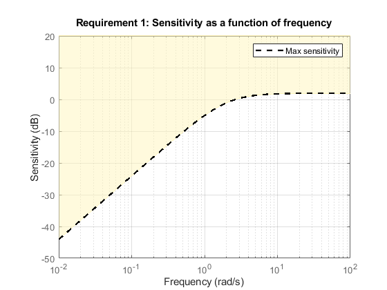
The first goal R1 specifies the desired profile for the sensitivity function. Sensitivity should be low at low frequency for good disturbance rejection. The second goal R2 imposes -20 dB/decade roll-off past 10 rad/s. The third goal R3 specifies the minimum decay, minimum damping, and maximum natural frequency for the closed-loop poles.
viewGoal(R1)
viewGoal(R2)
viewGoal(R3)
You can now use systune to robustly tune the PID gains, that is, to try and meet the design objectives for all possible values of the uncertain DC motor parameters. Because local minima may exist, perform three separate tunings from three different sets of initial gain values.
opt = systuneOptions('RandomStart',2);
rng(0), [CL,fSoft] = systune(CL0,[R1 R2 R3],opt);
Nominal tuning:
Design 1: Soft = 0.838, Hard = -Inf
Design 2: Soft = 0.838, Hard = -Inf
Design 3: Soft = 0.914, Hard = -Inf

Robust tuning of Design 2:
Soft: [0.838,2.01], Hard: [-Inf,-Inf], Iterations = 40
Soft: [0.875,1.76], Hard: [-Inf,-Inf], Iterations = 29
Soft: [0.935,2.77], Hard: [-Inf,-Inf], Iterations = 28
Soft: [1.35,1.35], Hard: [-Inf,-Inf], Iterations = 35
Final: Soft = 1.35, Hard = -Inf, Iterations = 132

Robust tuning of Design 1:
Soft: [0.838,1.96], Hard: [-Inf,-Inf], Iterations = 65
Soft: [0.875,1.76], Hard: [-Inf,-Inf], Iterations = 30
Soft: [1.02,2.98], Hard: [-Inf,-Inf], Iterations = 32
Soft: [1.34,1.36], Hard: [-Inf,-Inf], Iterations = 32
Soft: [1.35,1.35], Hard: [-Inf,-Inf], Iterations = 20
Final: Soft = 1.35, Hard = -Inf, Iterations = 179

Robust tuning of Design 3:
Soft: [0.914,2.37], Hard: [-Inf,-Inf], Iterations = 57
Soft: [0.875,1.76], Hard: [-Inf,-Inf], Iterations = 74
Soft: [1.02,2.98], Hard: [-Inf,-Inf], Iterations = 34
Soft: [1.34,1.36], Hard: [-Inf,-Inf], Iterations = 32
Soft: [1.35,1.35], Hard: [-Inf,-Inf], Iterations = 20
Final: Soft = 1.35, Hard = -Inf, Iterations = 217
The final value is close to 1 so the tuning goals are nearly achieved throughout the uncertainty range. The tuned PID controller is
showTunable(CL)
C =

             1            s
  Kp + Ki * --- + Kd * --------
             s          Tf*s+1

  with Kp = 33.8, Ki = 83.2, Kd = 2.34, Tf = 0.028

Name: C
Continuous-time PIDF controller in parallel form.
Next check how this PID rejects a step load disturbance for 30 randomly selected values of the uncertain parameters.
S = getSensitivity(CL,'dLoad');
clf, step(usample(S,30),getNominal(S),3)
title('Load disturbance rejection')
legend('Sampled uncertainty','Nominal')
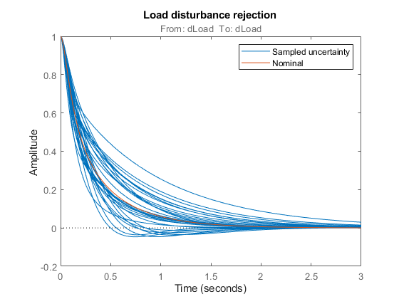
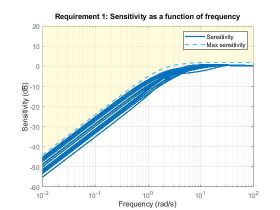
The rejection performance remains uniform despite large plant variations. You can also verify that the sensitivity function robustly stays within the prescribed bound.
viewGoal(R1,CL)
Robust tuning with systune is easy. Just include plant uncertainty in the tunable closed-loop model using ureal objects, and the software automatically tries to achieve the tuning goals for the entire uncertainty range.