Introduction to Model Predictive Path Integral (MPPI) Controller

Since R2026a

Model Predictive Path Integral (MPPI) control is an advanced Model Predictive Control (MPC)–based algorithm for motion planning in robotics and autonomous navigation. It is designed for complex, uncertain environments, where real-time adaptability is crucial. Unlike traditional deterministic approaches, MPPI formulates this process using stochastic optimal control, where control inputs are sampled from a distribution with a specified standard deviation to explore multiple future actions and identify the best one.

MPPI is particularly effective for:

Nonlinear dynamics, where motion isn’t simple or linear.
Non-convex objectives, multiple possible paths or goals.
Real-time decision-making in dynamic environments

By simulating many candidate trajectories, scoring them, and weighting the best ones, MPPI enables robots to avoid obstacles, maintain stability, and adapt to changing conditions.

MPPI Algorithm Structure

MPPI follows a structured process that includes:

Trajectory Generation — Sample control inputs from a predefined distribution and propagate them through the vehicle kinematics to generate a large set of candidate trajectories. This process uses stochastic sampling to explore diverse motion paths, enabling robust planning under uncertainty.
Cost Computation — Evaluate each trajectory based on predefined cost functions such as path adherence, obstacle avoidance, control smoothness.
Control Update — Assign higher weights to lower-cost (better) trajectories using a softmax function, then update the control sequence by computing a weighted average of all sampled control inputs. At each timestep, only the first control input from this updated sequence is applied to the system, and the process repeats at the next timestep. This iterative update allows better-performing trajectories to have a greater influence on the applied control action and drives convergence toward an optimal trajectory.

The path integral control theory computes the optimal trajectory by averaging control inputs weighted by their evaluations.

The image below shows a graphical overview of the MPPI algorithm in the form of a workflow chart.

Core Components of MPPI Algorithm

Trajectory Generation

In the first phase of MPPI, the algorithm generates possible future motion paths called trajectories, by sampling different control inputs and simulating how the system would move when applying each one.

Control Inputs Sampling — Samples a set of potential control sequences (u_[0,1], u_[0,2], ... u_[i,j]) from a predefined distribution to generate multiple candidate trajectories, where u_[i,j] represents the control input at time step j for the i^th trajectory. Each control sequence is generated by perturbing a nominal control input using noise sampled from a Gaussian distribution with a defined standard deviation. A higher standard deviation encourages broader exploration of the control space, allowing the system to consider a wider variety of motion paths, while a lower standard deviation favors more conservative and refined trajectories. Each sampled control sequence produces a unique candidate trajectory, and the diversity and distribution of these samples significantly influence the algorithm’s ability to find an optimal solution.
State Propagation — Applies the sampled control sequences to the vehicle model kinematics to propagate the state forward. x_[i,j] represents the state of the system at time step j for the i^th trajectory. The system propagates states using the sampled control sequences:
$x_{[i, j + 1]} = f (x_{[i, j]}, u_{[i, j]})$
This process models potential future motions, accounting for vehicle model kinematics.

Cost Computation

After propagating states, the algorithm evaluates the cost for each trajectory, which is a critical component of the MPPI algorithm. It assigns a cost to each trajectory based on a predefined function, guiding the algorithm in selecting the most optimal path. These cost functions include:

Reference Path Alignment — Encourages the trajectory to closely follow a predefined reference path, minimizing the deviation from the desired trajectory to improve path adherence and accuracy.
- Lookahead Strategy — Uses the concept of lookahead to optimize local trajectories while maintaining alignment with a global reference path typically generated by planners, such as RRT* or Hybrid A*. The global reference path serves as the backbone for local trajectory planning, ensuring the system progresses toward its overall destination. The key concepts of lookahead strategy include:
  - Lookahead Time — Duration, in seconds, used to compute the lookahead distance. A larger lookahead time enables the controller to plan further ahead, improving obstacle anticipation but increasing computation cost. A smaller lookahead time reduces reaction time to new obstacles but allows faster controller updates.
  - Lookahead Distance — Segment of the global reference path that the controller considers for local planning during each iteration. The controller determines the lookahead distance by multiplying the vehicle’s maximum forward velocity with the lookahead time.
  - Lookahead Point — Specific pose on the global reference path located at the lookahead distance from the current position of the vehicle. This point acts as a local target for trajectory optimization.
  - Lookahead Poses — Poses on the global reference path between the vehicle’s current position and the lookahead point. These poses define the trajectory segment under consideration and guide the controller in maintaining alignment with the global path.
  This mechanism enables real-time trajectory adjustments and resembles concepts in the Pure Pursuit Algorithm, emphasizing adaptability to dynamic environments.
- Following Cost — Encourages the trajectory to move towards the lookahead point and maintain progress toward the target.
- Alignment Cost — Focuses on aligning the trajectory with the lookahead poses, minimizing lateral deviations and ensuring the vehicle’s orientation is consistent with the reference path.
Obstacle Avoidance — Incorporates obstacle avoidance into the cost computation by penalizing trajectories that approach obstacles, with higher costs assigned to near-collision states. The cost function is an exponential decay function that is calculated based on the distance from the closest obstacle.
Control Smoothing — Penalizes sharp changes in velocity or direction, promoting smoother trajectories. This reduces erratic movements and supports energy-efficient, stable motion.

Iterative Update

Each cost function component is assigned a weight to balance the influence of different factors. The final trajectory cost is computed as:

$J_{i} = c_{1} C_{1}^{i} + c_{2} C_{2}^{i} + c_{3} C_{3}^{i} + ... + c_{n} C_{n}^{i}$

where,

Cⁱ_n represents different cost function components, such as obstacle avoidance, reference path alignment, and smoothness. n represents the number of cost function component involved.
c_n is the respective weight assigned to the cost function components for the i^th trajectory.

A probability weight is then assigned to each trajectory using the formula:

$w_{i} = e^{- (J_{i} / λ)}$

where,

w — Weight assigned to the trajectory, determining its likelihood of being selected in the optimization process. A higher weight implies a higher probability of selection, while a lower weight decreases the chances of that trajectory being chosen.
e — The base of the natural logarithm (approximately 2.718), which is used in the exponential function to scale the influence of the cost term.
J — The cost of the trajectory, computed as the sum of penalties from various factors, including obstacle avoidance, reference path alignment, path smoothness, and custom constraints. The cost reflects how well the trajectory adheres to the defined objectives.
λ — Key tuning parameter that controls how sensitive the trajectory weighting is to cost differences in MPPI:
- High λ — Produces more uniform trajectory weights, encouraging exploration by allowing a wider range of trajectories to influence the control decision. This setting is useful in uncertain or dynamic environments where diverse path options should be considered.
- Low λ — Increases sensitivity to cost differences, so lower-cost (better) trajectories dominate the weighting. This setting favors exploitation, resulting in more precise and reliable path following when accuracy is critical.
The λ parameter thus allows for a dynamic adjustment between exploration and exploitation, enabling MPPI to adapt the trajectory selection process based on the operational requirements of the robot and its environment. the diagram below represents how different values of λ influences the probability weight: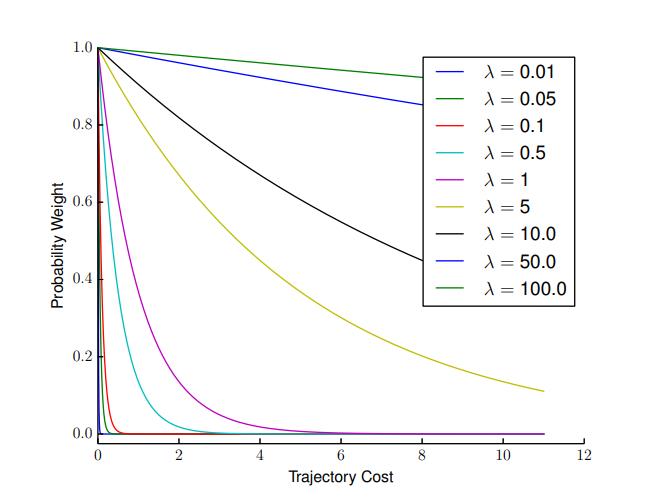

The final optimal control is generated by averaging the control inputs across trajectories, weighted by their assigned probability:

$U = \sum_{i}^{} w_{i} U_{i}$

This step ensures that the chosen trajectory balances robustness, path adherence, and smoothness. MPPI iterates through this process in real-time, continuously refining its trajectory selection based on new sensor data and system feedback.

Significance of MPPI in Offroad Autonomy

MPPI is well-suited for offroad autonomy due to its ability to handle complex dynamics, uncertainty, and even non-differentiable cost functions:

Ability to Handle Non-Differentiable Cost Functions — MPPI can work with non-differentiable cost functions, such as those derived from traversability maps, thanks to its stochastic optimal nature. This capability is critical because many traditional optimization-based algorithms struggle with such cost structures.
Navigation of Constrained Environments — Helps vehicles steer through tight spaces, such as sharp turns, steep slopes, and narrow paths. It adapts in real time to maintain safe and stable movement, even in fast-changing environments like mining sites.
Adaptive Speed and Traction Control — Adjusts speed and acceleration based on engine power limits and traction needs. This helps the vehicle move smoothly and safely on difficult terrains, including loose soil or steep climbs.
Resilience to Changing Terrain — Handles variability such as offroad terrain changes due to rocks, inclines, or soft ground, by accounting for nonlinear dynamics and random disturbances, making the motion of the vehicle more reliable.
Scalability for High-Dimensional Control Spaces — Supports systems with many control inputs, such as multi-axle vehicles or articulated machines. It also lets users define custom cost functions to focus on specific goals like energy savings, safety, or precision.
Real-Time Implementation — Quickly generates valid paths that meet the timing needs of real-world systems. This real-time responsiveness keeps the vehicle stable and accurate during complex maneuvers.

Challenges

The benefits of the MPPI controller are accompanied by certain challenges such as:

Parameter Sensitivity — The algorithm’s performance depends on choosing suitable parameters, such as the number of sampled trajectories and their distribution.
Computational Cost — Real-time implementation requires efficient computation, which can be resource-intensive for high-dimensional systems.
Tuning — Adjusting cost function parameters and the λ sensitivity parameter may require iterative experimentation to achieve optimal results.

References

[1] Williams, Grady, Paul Drews, Brian Goldfain, James M. Rehg, and Evangelos A. Theodorou. “Aggressive Driving with Model Predictive Path Integral Control.” In 2016 IEEE International Conference on Robotics and Automation (ICRA), 1433–40. Stockholm: IEEE, 2016. https://doi.org/10.1109/ICRA.2016.7487277.