creditMigrationCopula Simulation Workflow

This example shows a common workflow for using a creditMigrationCopula object for a portfolio of counterparty credit ratings.

Step 1. Create a creditMigrationCopula object with a 4-factor model

Load the saved portfolio data.

load CreditMigrationData.mat;

Scale the bond prices for portfolio positions for each bond.

migrationValues = migrationPrices .* numBonds;

Create a creditMigrationCopula object with a 4-factor model using creditMigrationCopula.

cmc = creditMigrationCopula(migrationValues,ratings,transMat,...
lgd,weights,'FactorCorrelation',factorCorr)

cmc = 
  creditMigrationCopula with properties:

            Portfolio: [250x5 table]
    FactorCorrelation: [4x4 double]
         RatingLabels: [8x1 string]
     TransitionMatrix: [8x8 double]
             VaRLevel: 0.9500
          UseParallel: 0
      PortfolioValues: []

Step 2. Set the VaRLevel to 99%.

Set the VarLevel property for the creditMigrationCopula object to 99% (the default is 95%).

 cmc.VaRLevel = 0.99;

Step 3. Display the Portfolio property for information about migration values, ratings, LGDs, and weights.

Display the Portfolio property containing information about migration values, ratings, LGDs, and weights. The columns in the migration values are in the same order of the ratings, with the default rating in the last column.

 head(cmc.Portfolio)

    ID                                  MigrationValues                                   Rating     LGD                    Weights              
    __    ____________________________________________________________________________    ______    ______    ___________________________________

    1      13301     13280     13216     13082     12421     11939     10180     11700    "A"       0.6509      0       0       0     0.5     0.5
    2       2944      2939    2923.8    2892.6    2737.1      2624    2218.2      3000    "BBB"     0.8283      0    0.55       0       0    0.45
    3     9797.5    9787.9    9754.2    9681.2    9320.5      9050    7976.8      9100    "AA"      0.6041      0     0.7       0       0     0.3
    4     4760.4    4754.3    4735.7    4696.9    4502.7    4359.7    3824.8      4400    "BB"      0.6509      0    0.55       0       0    0.45
    5      10524     10509     10466     10376    9923.5    9591.5    8362.1     10100    "BBB"     0.4966      0       0    0.75       0    0.25
    6     6192.8    6183.2    6154.2    6094.3    5795.1    5576.4    4782.7      6200    "BB"      0.8283      0       0       0    0.65    0.35
    7     5736.9    5727.5    5699.3    5640.7    5349.5    5137.6    4367.4      5200    "BB"      0.6041      0       0       0    0.65    0.35
    8     5065.3    5062.7    5056.4    5038.8    4956.2    4892.2    4491.9      4800    "BB"      0.4873    0.5       0       0       0     0.5

Step 4. Display migration values for a counterparty.

For example, you can display the migration values for the first counterparty. Note that the value for default is higher than some of the non-default ratings. This is because the migration value for the default rating is a reference value (for example, face value, forward value at current rating, or other) that is multiplied by the recovery rate during the simulation to get the value of the asset in the event of default. The recovery rate is 1-LGD when the LGD input to creditMigrationCopula is a constant LGD value (the LGD input has one column). The recovery rate is a random quantity when the LGD input to creditMigrationCopula is specified as a mean and standard deviation for a beta distribution (the LGD input has two columns).

bar(cmc.Portfolio.MigrationValues(1,:))
xticklabels(cmc.RatingLabels)
title('Migration Values for First Company')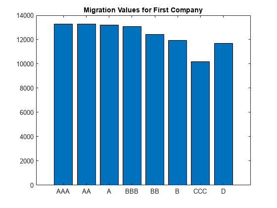

Step 5. Run a simulation.

Use the simulate function to simulate 100,000 scenarios.

 cmc = simulate(cmc,1e5)

cmc = 
  creditMigrationCopula with properties:

            Portfolio: [250x5 table]
    FactorCorrelation: [4x4 double]
         RatingLabels: [8x1 string]
     TransitionMatrix: [8x8 double]
             VaRLevel: 0.9900
          UseParallel: 0
      PortfolioValues: [2.0082e+06 1.9950e+06 1.9933e+06 2.0009e+06 1.9819e+06 1.9955e+06 1.9962e+06 1.9966e+06 2.0018e+06 2.0036e+06 1.9873e+06 1.9929e+06 2.0015e+06 1.9875e+06 1.9962e+06 2.0070e+06 2.0054e+06 2.0037e+06 ... ] (1x100000 double)

Step 6. Generate a report for the portfolio risk.

Use the portfolioRisk function to obtain a report for risk measures and confidence intervals for EL, Std, VaR, and CVaR.

[portRisk,RiskConfidenceInterval] = portfolioRisk(cmc)

portRisk=1×4 table
      EL       Std      VaR     CVaR 
    ______    _____    _____    _____

    4515.9    12963    57176    83975

RiskConfidenceInterval=1×4 table
           EL                Std               VaR               CVaR     
    ________________    ______________    ______________    ______________

    4435.6    4596.3    12907    13021    55739    58541    82137    85812

Step 7. Visualize the distribution.

View a histogram of the portfolio values.

figure
h = histogram(cmc.PortfolioValues,125);
title('Distribution of Portfolio Values');

Step 8. Overlay the value if all counterparties maintain current credit ratings.

Overlay the value that the portfolio object (cmc) takes if all counterparties maintain their current credit ratings.

CurrentRatingValue = portRisk.EL + mean(cmc.PortfolioValues);
 
hold on
plot([CurrentRatingValue CurrentRatingValue],[0 max(h.Values)],'LineWidth',2);
grid on

Step 9. Generate a risk contributions report.

Use the riskContribution function to display the risk contribution. The risk contributions, EL and CVaR, are additive. If you sum each of these two metrics over all the counterparties, you get the values reported for the entire portfolio in the portfolioRisk table.

rc = riskContribution(cmc);
disp(rc(1:10,:))

    ID      EL       Std       VaR       CVaR 
    __    ______    ______    ______    ______

     1    15.521    41.153    238.72    279.18
     2      8.49    18.838    92.074    122.19
     3    6.0937    20.069    113.22    181.53
     4    6.6964    55.885    272.23    313.25
     5    23.583    73.905    360.32    573.39
     6    10.722    114.97    445.94    728.38
     7    1.8393    84.754    262.32    490.39
     8    11.711    39.768    175.84    253.29
     9    2.2154    4.4038    22.797    31.039
    10    1.7453    2.5545    9.8801    17.603

Step 10. Simulate the risk exposure with a t copula.

To use a t copula with 10 degrees of freedom, use the simulate function with optional input arguments. Save the results to a new creditMigrationCopula object (cmct).

cmct = simulate(cmc,1e5,'Copula','t','DegreesOfFreedom',10)

cmct = 
  creditMigrationCopula with properties:

            Portfolio: [250x5 table]
    FactorCorrelation: [4x4 double]
         RatingLabels: [8x1 string]
     TransitionMatrix: [8x8 double]
             VaRLevel: 0.9900
          UseParallel: 0
      PortfolioValues: [2.0021e+06 2.0007e+06 1.9834e+06 2.0025e+06 2.0002e+06 2.0021e+06 2.0039e+06 2.0023e+06 2.0017e+06 2.0101e+06 2.0002e+06 2.0080e+06 2.0007e+06 2.0052e+06 1.9969e+06 2.0071e+06 2.0045e+06 1.9979e+06 ... ] (1x100000 double)

Step 11. Generate a report for the portfolio risk for the t copula.

Use the portfolioRisk function to obtain a report for risk measures and confidence intervals for EL, Std, VaR, and CVaR.

[portRisk2,RiskConfidenceInterval2] = portfolioRisk(cmct)

portRisk2=1×4 table
     EL      Std      VaR        CVaR   
    ____    _____    _____    __________

    4544    17034    72270    1.2391e+05

RiskConfidenceInterval2=1×4 table
           EL                Std               VaR                    CVaR          
    ________________    ______________    ______________    ________________________

    4438.5    4649.6    16960    17109    69769    75382    1.1991e+05    1.2791e+05

Step 12. Visualize the distribution for the t copula.

View a histogram of the portfolio values.

figure
h = histogram(cmct.PortfolioValues,125);
title('Distribution of Portfolio Values for t Copula');

Step 13. Overlay the value if all counterparties maintain current credit ratings for t copula.

Overlay the value that the portfolio object (cmct) takes if all counterparties maintain their current credit ratings.

CurrentRatingValue2 = portRisk2.EL + mean(cmct.PortfolioValues);

hold on
plot([CurrentRatingValue2 CurrentRatingValue2],[0 max(h.Values)],'LineWidth',2);
grid on