Operations with RF Data Objects
This example shows you how to manipulate RF data directly using rfdata objects. First, you create an rfdata.data object by reading in the S-parameters of a two-port passive network stored in the Touchstone format data file, passive.s2p. Next, you create a circuit object, rfckt.amplifier, and you update the properties of this object using three data objects.
Read Touchstone Data File
Use the read method of the rfdata.data object to read the Touchstone data file passive.s2p. The parameters in this data file are the 50-Ohm S-parameters of a 2-port passive network at frequencies ranging from 315 kHz to 6.0 GHz.
data = rfdata.data;
data = read(data,"passive.s2p")
data =
rfdata.data with properties:
Freq: [202×1 double]
S_Parameters: [2×2×202 double]
GroupDelay: [202×1 double]
NF: [202×1 double]
OIP3: [202×1 double]
Z0: 50.0000 + 0.0000i
ZS: 50.0000 + 0.0000i
ZL: 50.0000 + 0.0000i
IntpType: 'Linear'
Name: 'Data object'
Use the extract method of the rfdata.data object to get other network parameters. For example, here are the frequencies, 75-Ohm S-parameters, and Y-parameters which are converted from the original 50-Ohm S-parameters in passive.s2p data file.
[s_params,freq] = extract(data,'S_PARAMETERS',75);
y_params = extract(data,'Y_PARAMETERS');
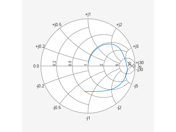
Use the RF utility function, smithplot to plot the 75-Ohm S11 on a Smith® Chart.
s11 = s_params(1,1,:);
figure
smithplot(freq, s11(:))
Here are the four 75-Ohm S-parameters and four Y-parameters at 6.0 GHz, the last frequency.
f = freq(end)
f =
6.0000e+09
s = s_params(:,:,end)
s = 2×2 complex

  -0.0764 - 0.5401i   0.6087 - 0.3018i
   0.6094 - 0.3020i  -0.1211 - 0.5223i
y = y_params(:,:,end)
y = 2×2 complex

   0.0210 + 0.0252i  -0.0215 - 0.0184i
  -0.0215 - 0.0185i   0.0224 + 0.0266i
Create RF Data Objects for Amplifier with Your Own Data
In this example, you create a circuit object, rfckt.amplifier. Then you create three data objects and use them to update the properties of the circuit object.
The rfckt.amplifier object has properties for network parameters, noise data and nonlinear data:
NetworkDatais anrfdata.networkobject for network parameters.NoiseDatais for noise parameters which could be a scalar NF (dB), anrfdata.noise, or anrfdata.nfobject.NonlinearDatais for nonlinear parameters which could be a scalar OIP3 (dBm), anrfdata.power, or anrfdata.ip3object.
By default, these properties of rfckt.amplifier contain data from the default.amp data file. NetworkData is an rfdata.network object that contains 50-Ohm 2-port S-Parameters at 191 frequencies ranging from 1.0 GHz to 2.9 GHz. NoiseData is an rfdata.noise object that contains spot noise data at 9 frequencies ranging from 1.9 GHz to 2.48 GHz. The NonlinearData parameter is an rfdata.power object that contains Pin/Pout data at 2.1 GHz.
amp = rfckt.amplifier
amp =
   rfckt.amplifier with properties:

         NoiseData: [1×1 rfdata.noise]
     NonlinearData: [1×1 rfdata.power]
          IntpType: 'Linear'
       NetworkData: [1×1 rfdata.network]
             nPort: 2
    AnalyzedResult: [1×1 rfdata.data]
              Name: 'Amplifier'
Use the following code to create an rfdata.network object that contains 2-port Y-parameters of an amplifier at 2.08 GHz, 2.10 GHz and 2.15 GHz. Later in this example, you use this data object to update the NetworkData property of the amplifier object.
f = [2.08 2.10 2.15] * 1.0e9;
y(:,:,1) = [-.0090-.0104i, .0013+.0018i; -.2947+.2961i, .0252+.0075i];
y(:,:,2) = [-.0086-.0047i, .0014+.0019i; -.3047+.3083i, .0251+.0086i];
y(:,:,3) = [-.0051+.0130i, .0017+.0020i; -.3335+.3861i, .0282+.0110i];
netdata = rfdata.network('Type','Y_PARAMETERS','Freq',f,'Data',y)
netdata =
   rfdata.network with properties:

    Type: 'Y_PARAMETERS'
    Freq: [3×1 double]
    Data: [2×2×3 double]
      Z0: 50.0000 + 0.0000i
    Name: 'Network parameters'
Use the following code to create an rfdata.nf object that contains noise figures of the amplifier, in dB, at seven frequencies ranging from 1.93 GHz to 2.40 GHz. Later in this example, you use this data object to update the NoiseData property of the amplifier object.
f = [1.93 2.06 2.08 2.10 2.15 2.3 2.4] * 1.0e+009;
nf = [12.4521 13.2466 13.6853 14.0612 13.4111 12.9499 13.3244];
nfdata = rfdata.nf('Freq',f,'Data',nf)
nfdata =
   rfdata.nf with properties:

    Freq: [7×1 double]
    Data: [7×1 double]
    Name: 'Noise figure'
Use the following code to create an rfdata.ip3 object that contains the output third-order intercept points of the amplifier, which is 8.45 watts at 2.1 GHz. Later in this example, you use this data object to update the NonlinearData property of the amplifier object.
ip3data = rfdata.ip3('Type','OIP3','Freq',2.1e9,'Data',8.45)
ip3data =
   rfdata.ip3 with properties:

    Type: 'OIP3'
    Freq: 2.1000e+09
    Data: 8.4500
    Name: '3rd order intercept'
Use the following code to update the properties of the amplifier object with three data objects you created in the previous steps. To get a good amplifier object, the data in these data objects must be accurate. These data could be obtained from RF measurements, or circuit simulation using other tools.
amp.NetworkData = netdata;
amp.NoiseData = nfdata;
amp.NonlinearData = ip3data
amp =
   rfckt.amplifier with properties:

         NoiseData: [1×1 rfdata.nf]
     NonlinearData: [1×1 rfdata.ip3]
          IntpType: 'Linear'
       NetworkData: [1×1 rfdata.network]
             nPort: 2
    AnalyzedResult: [1×1 rfdata.data]
              Name: 'Amplifier'