Train DDPG Agent for Adaptive Cruise Control

This example uses:

This example shows how to train a deep deterministic policy gradient (DDPG) agent for adaptive cruise control (ACC) in Simulink®. For more information on DDPG agents, see Deep Deterministic Policy Gradient (DDPG) Agent.

Fix Random Seed Generator to Improve Reproducibility

The example code might involve computation of random numbers at several stages. Fixing the random number stream at the beginning of some sections in the example code preserves the random number sequence in the section every time you run it, which increases the likelihood of reproducing the results. For more information, see Results Reproducibility.

Fix the random number stream with seed 0 and random number algorithm Mersenne Twister. For more information on controlling the seed used for random number generation, see rng.

previousRngState = rng(0,"twister");

The output previousRngState is a structure that contains information about the previous state of the stream. You will restore the state at the end of the example.

Adaptive Cruise Control Simulink Model

The reinforcement learning environment for this example is the simple longitudinal dynamics for an ego car and lead car. The training goal is to make the ego car travel at a set velocity while maintaining a safe distance from lead car by controlling longitudinal acceleration and braking. This example uses the same vehicle model as the Adaptive Cruise Control System Using Model Predictive Control (Model Predictive Control Toolbox) example.

Specify the initial position and velocity for the two vehicles.

x0_lead = 50;   % initial position for lead car (m)
v0_lead = 25;   % initial velocity for lead car (m/s)
x0_ego = 10;    % initial position for ego car (m)
v0_ego = 20;    % initial velocity for ego car (m/s)

Specify standstill default spacing (m), time gap (s) and driver-set velocity (m/s).

D_default = 10;
t_gap = 1.4;
v_set = 30;

To simulate the physical limitations of the vehicle dynamics, constraint the acceleration to the range [–3,2] m/s^2.

amin_ego = -3;
amax_ego = 2;

Define the sample time Ts and simulation duration Tf in seconds.

Ts = 0.1;
Tf = 60;

Open the model.

mdl = "rlACCMdl";
open_system(mdl)
agentblk = mdl + "/RL Agent";

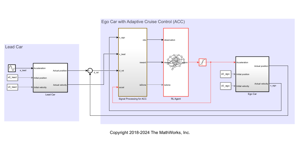
In this model:

The acceleration action signal from the agent to the environment is from –3 to 2 m/s^2.
The reference velocity for the ego car $V_{r e f}$ is defined as follows. If the relative distance is less than the safe distance, the ego car tracks the minimum of the lead car velocity and driver-set velocity. In this manner, the ego car maintains some distance from the lead car. If the relative distance is greater than the safe distance, the ego car tracks the driver-set velocity. In this example, the safe distance is defined as a linear function of the ego car longitudinal velocity $V$ ; that is, $t_{g a p} * V + D_{d e f a u l t}$ . The safe distance determines the reference tracking velocity for the ego car.
The observations from the environment are the velocity error $e = V_{r e f} - V_{e g o}$ , its integral $\int e$ , and the ego car longitudinal velocity $V$ .
The simulation is terminated when longitudinal velocity of the ego car is less than 0, or the relative distance between the lead car and ego car becomes less than 0.
The reward $r_{t}$ , provided at every time step $t$ , is

$r_{t} = - (0.1 e_{t}^{2} + u_{t - 1}^{2}) + M_{t}$

where $u_{t - 1}$ is the control input from the previous time step. The logical value $M_{t} = 1$ if velocity error $e_{t}^{2} < = 0.25$ ; otherwise, $M_{t} = 0$ .

Create Environment Object

Create a reinforcement learning environment object for the model.

Create the observation specification.

obsInfo = rlNumericSpec([3 1], ...
    LowerLimit=-inf*ones(3,1), ...
    UpperLimit=inf*ones(3,1));
obsInfo.Name = "observations";
obsInfo.Description = "velocity error and ego velocity";

Create the action specification.

actInfo = rlNumericSpec([1 1], ...
    LowerLimit=-3,UpperLimit=2);
actInfo.Name = "acceleration";

Create the environment object.

env = rlSimulinkEnv(mdl,agentblk,obsInfo,actInfo);

To define the initial condition for the position of the lead car, specify the reset function localResetFcn, which is defined at the end of the example.

env.ResetFcn = @localResetFcn;

Create Default DDPG Agent

You will create and train a DDPG agent in this example. The agent uses:

A Q-value function critic to estimate the value of the policy. The critic takes the current observation and an action as inputs and returns a single scalar as output (the estimated discounted cumulative long-term reward given the action from the state corresponding to the current observation, and following the policy thereafter).
A deterministic policy over a continuous action space, which is learned by a continuous deterministic actor. This actor takes the current observation as input and returns as output an action that is a deterministic function of the observation.

The actor and critic functions are approximated using neural network representations. Create an agent initialization object to initialize the networks with the hidden layer size 200.

initOpts = rlAgentInitializationOptions(NumHiddenUnit=200);

Configure the hyperparameters for training using rlDDPGAgentOptions.

Specify a mini-batch size of 50. Smaller mini-batches are computationally efficient but might introduce variance in training. By contrast, larger batch sizes can make the training stable but require higher memory.
Specify the actor and critic learning rates as 3e-4 and 1e-2. A large learning rate causes drastic updates which might lead to divergent behaviors, while a low value might require many updates before reaching the optimal point.
Specify the sample time as Ts.

Specify the actor and critic optimizer options.

actorOptions = rlOptimizerOptions( ...
    LearnRate                 = 3e-4, ...
    GradientThreshold         = 1, ...
    L2RegularizationFactor    = 1e-4);

criticOptions = rlOptimizerOptions( ...
    LearnRate                 = 1e-2, ...
    GradientThreshold         = 1, ...
    L2RegularizationFactor    = 1e-4);

Create the agent options object. For more information, see rlDDPGAgentOptions.

agentOptions = rlDDPGAgentOptions( ...
    SampleTime                = Ts, ...
    MiniBatchSize             = 50, ...
    ActorOptimizerOptions     = actorOptions, ...
    CriticOptimizerOptions    = criticOptions, ...
    ExperienceBufferLength    = 1e6);

The DDPG agent in this example uses an Ornstein-Uhlenbeck (OU) noise model for exploration. For the noise model:

Specify a mean attraction value of 0.7. A larger mean attraction value keeps the noise values close to the mean.
Specify a standard deviation value of 0.4 to improve exploration during training.
Specify a decay rate of 1e-5 for the standard deviation. The decay causes exploration to reduce gradually as the training progresses.

agentOptions.NoiseOptions.MeanAttractionConstant     = 0.7;
agentOptions.NoiseOptions.StandardDeviation          = 0.4;
agentOptions.NoiseOptions.StandardDeviationDecayRate = 1e-5;

Create the DDPG agent using the observation and action input specifications, initialization options and agent options. When you create the agent, the initial parameters of the actor and critic networks are initialized with random values. Fix the random number stream so that the agent is always initialized with the same parameter values.

rng(0,"twister");
agent = rlDDPGAgent(obsInfo,actInfo,initOpts,agentOptions);

For more information, see rlDDPGAgent.

Train Agent

To train the agent, first specify the training options. For this example, use the following options:

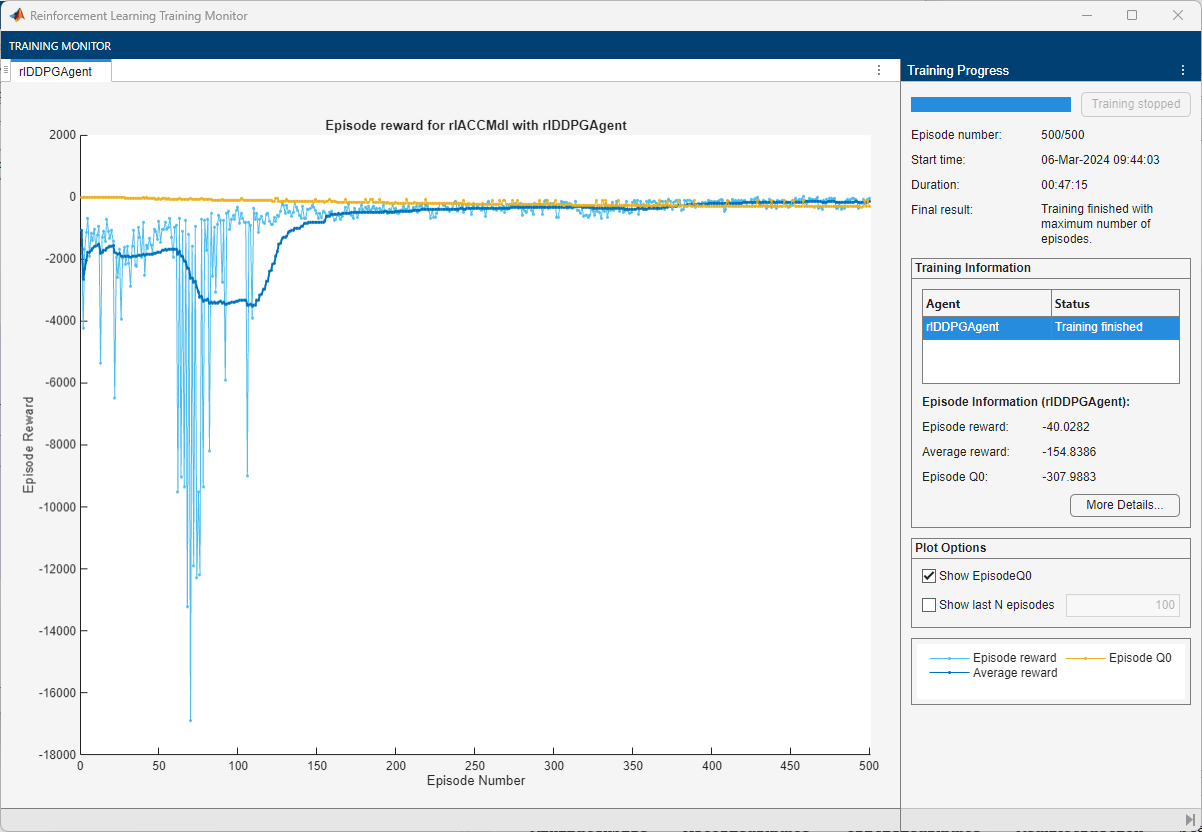
Run the training episode for 500 episodes, with each episode lasting a maximum of maxsteps time steps.
Display the training progress in the Reinforcement Learning Training Monitor window.

For more information on training options, see rlTrainingOptions.

maxepisodes = 500;
maxsteps = ceil(Tf/Ts);
trainingOpts = rlTrainingOptions( ...
    MaxEpisodes          = maxepisodes, ...
    MaxStepsPerEpisode   = maxsteps, ...
    Plots                = "training-progress", ...
    StopTrainingCriteria = "none");

Fix the random stream for reproducibility.

rng(0,"twister");

Train the agent using the train function. Training is a computationally intensive process that takes several minutes to complete. To save time while running this example, load a pretrained agent by setting doTraining to false. To train the agent yourself, set doTraining to true.

doTraining = false;
if doTraining    
    % Train the agent.
    trainResult = train(agent,env,trainingOpts);
else
    % Load a pretrained agent for the example.
    load("SimulinkACCDDPG.mat","agent")
end

An example of the training is shown below. The actual results might vary because of randomness in the training process.

Simulate Agent

Fix the random stream for reproducibility.

rng(0,"twister");

By default, the agent uses a greedy (hence deterministic) policy in simulation. To use the exploratory policy instead, set the UseExplorationPolicy agent property to true.

To validate the performance of the trained agent deterministically, set the initial position of the lead car to 80 (m) and simulate the model. To validate the performance for a randomly chosen initial position, set useRandomInitialConditions to true.

useRandomInitialConditions = false;
if useRandomInitialConditions
    % The simulink sim function uses the workspace value of x0_lead
    x0_lead = 80;
    sim(mdl);
else
    % The reinforcement learning sim function 
    % randomizes the value of x0_lead
    simOptions = rlSimulationOptions(MaxSteps=maxsteps);
    experience = sim(env,agent,simOptions);
end

For more information on agent simulation, see rlSimulationOptions and sim.

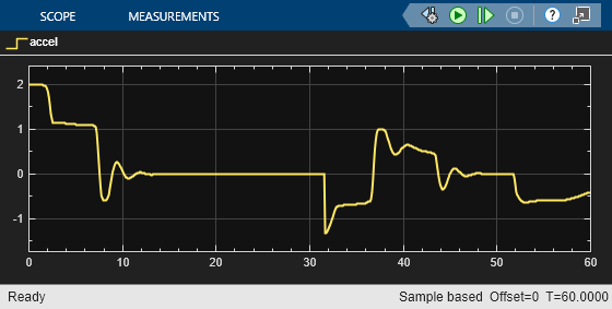
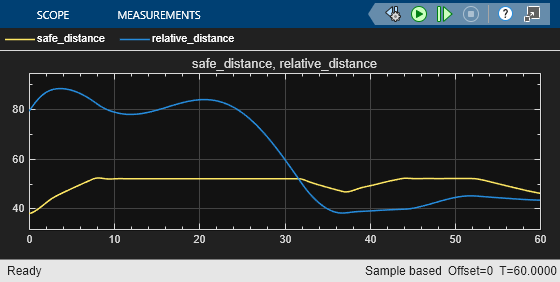
These plots show deterministic simulation results when lead car is initially 80 (m) ahead of the ego car.

In the first 30 seconds, the relative distance is greater than the safe distance (middle plot), so the ego car tracks the set velocity (bottom plot). To speed up and reach the set velocity, acceleration is initially positive (top plot).
At approximately 8 seconds, the ego car is able to track the set velocity and acceleration is reduced to zero.
After 30 seconds, the relative distance is less than the safe distance (middle plot), so the ego car tracks the minimum of the lead velocity and set velocity. To slow down and track the lead car velocity, the acceleration turns negative (top plot).
Throughout the simulation the ego car adjusts its acceleration to keep on tracking either the minimum between the lead velocity and the set velocity, or the set velocity, depending on whether the relative distance is deemed to be safe or not.

Restore the random number stream using the information stored in previousRngState.

rng(previousRngState);

Reset Function

The sim function calls the reset function at the start of each simulation episode, and the train function calls it at the start of each training episode. The reset function takes as input, and returns as output, a Simulink.SimulationInput (Simulink) object. The output object specifies temporary changes applied to model, which are then discarded when the simulation or training completes. For this example, the function localResetFcn uses the setVariable (Simulink) function to randomly set the variable x0_lead in the model workspace. For more information, see Reset Function for Simulink Environments.

function in = localResetFcn(in)
% Reset the initial position of the lead car.
in = setVariable(in,"x0_lead",40+randi(60,1,1));
end

Train DDPG Agent for Adaptive Cruise Control

Fix Random Seed Generator to Improve Reproducibility

Adaptive Cruise Control Simulink Model

Create Environment Object

Create Default DDPG Agent

Train Agent

Simulate Agent

Reset Function

See Also

Functions

Objects

Blocks

Topics