Main Content

radarpropfactor

One-way radar propagation factor

Since R2021a

Description

F = radarpropfactor(R,freq,ANHT) calculates the one-way propagation factor assuming a surface target and a sea state of 0. The calculation estimates the complex relative permittivity (dielectric constant) of the reflecting surface using a sea water model described in [1] that is valid from 100 MHz to 10 GHz. The target height is assumed to be the height of significant clutter sources above the average surface height. Specifically, the target height is calculated as 3 times the standard deviation of the surface height. Assuming the paths are the same, the two-way propagation factor is 2F. Atmospheric refraction is taken into account through the use of an EffectiveEarthRadius that can be specified. Scattering and ducting are assumed to be negligible.

F = radarpropfactor(___,TGTHT) calculates the target propagation factor assuming a target height of TGTHT.

example

F = radarpropfactor(___,Name,Value) allows you to specify additional input parameters as Name-Value arguments. You can specify additional name-value pair arguments in any order. This syntax can use any of the input arguments in the previous syntax.

radarpropfactor(___) plots the one-way propagation factor in dB versus range in km. Default range units are km.

Examples

collapse all

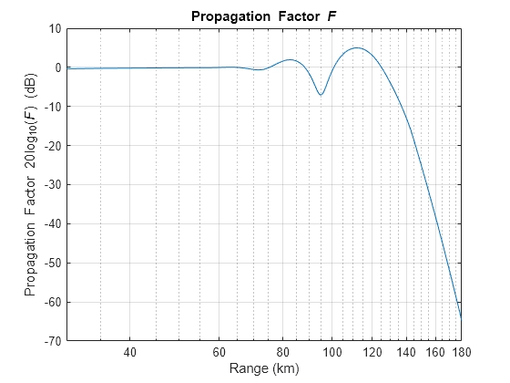
Plot the propagation factor for a 3 GHz S-band radar assuming an antenna height of 10 m and a target height of 1 km. Assume that the surface has a height standard deviation of 1 m, and the surface slope is 0.05 degrees.

R     = (30:0.5:180)*1e3; % Range (m)
freq  = 3e9;              % Frequency (Hz)
anht  = 10;               % Radar height (m)
tgtht = 1e3;              % Target height (m)
hgtsd = 1;                % Height standard deviation (m)
beta0 = 0.05;             % Surface slope (deg)

radarpropfactor(R,freq,anht,tgtht,...
    'SurfaceHeightStandardDeviation',hgtsd,...
    'SurfaceSlope',beta0)

ans = 301×1

   -0.3696
   -0.3566
   -0.3439
   -0.3316
   -0.3197
   -0.3082
   -0.2970
   -0.2862
   -0.2756
   -0.2654
      ⋮

Input Arguments

collapse all

Free space range, specified as a scalar or an M-length real vector. Units are in meters.

Example: 0.5

Data Types: single | double

Radar frequency in Hz, specified as a positive real scalar.

Data Types: double

Antenna height as referenced from the surface, specified as a positive scalar. Units are in meters.

Data Types: double

Target height as referenced from the surface, specified as a positive scalar. Units are in meters.

Data Types: double

Name-Value Arguments

Specify optional pairs of arguments as Name1=Value1,...,NameN=ValueN, where Name is the argument name and Value is the corresponding value. Name-value arguments must appear after other arguments, but the order of the pairs does not matter.

Before R2021a, use commas to separate each name and value, and enclose Name in quotes.

Example: 'SurfaceHeightStandardDeviation',hgtsd,'SurfaceSlope',beta0

Polarization of the transmitted wave, specified as 'H' or 'V'. 'H' indicates horizontal polarization and 'V' indicates vertical polarization.

Complex relative permittivity (dielectric constant) of the reflecting surface, specified as a complex scalar. The default value of dielectric constant depends on the value of the freq argument. The function uses a sea water model in [1] that is valid up to 10 GHz.

Data Types: single | double
Complex Number Support: Yes

Standard deviation of the surface height in meters, specified as positive scalar. The default value of 0.01 m indicates a sea state of 0. Units are in meters.

Data Types: single | double

Surface slope, specified as a nonnegative scalar. This value is expected to be 1.4 times the RMS surface slope. Given the condition that

2 × GRAZ/β0 < 1,

where GRAZ is the grazing angle of the geometry specified in degrees and β0 is the surface slope, the effective surface height standard deviation in meters is calculated as

Effective HGTSD = HGTSD × (2 × GRAZ/β0)1/5.

This calculation better accounts for shadowing. Otherwise, the effective height standard deviation is equal to HGTSD. This argument defaults to the surface slope value output by the searoughness function for a sea state of 0. Units are in degrees.

Data Types: double

Surface vegetation type, specified as 'Trees', 'Weeds', and 'Brush' are assumed to be dense vegetation. 'Grass' is assumed to be thin grass. Use this argument when using the function on surfaces different from the sea.

Half-power elevation beamwidth in degrees, specified as a scalar between 0° and 90°. The elevation beamwidth is used in the calculation of a sinc antenna pattern. The default antenna pattern is symmetric with respect to the beam maximum and is of the form sin(u)/u. The parameter u is given by u = k sin(θ), where θ is the elevation angle in radians and k is given by k = x0 / sin(π × ELBW/360), where ELBW is the half-power elevation beamwidth and x0 ≈ 1.3915573 is a solution of sin(x) = x/√2.

Data Types: double

Antenna elevation pattern, specified as a real-valued column vector. Values for 'AntennaPattern' must be specified together with values for 'PatternAngles'. Both vectors must have the same size. If both an antenna pattern and an elevation beamwidth are specified, radarpropfactor uses the antenna pattern and ignores the elevation beamwidth value. This argument defaults to a sinc antenna pattern.

Example: cosd([–90:90])

Data Types: double

Antenna pattern elevation angles specified as a real-valued column vector. The size of the vector specified by PatternAngles must be the same as that specified by AntennaPattern. Angle units are expressed in degrees and must lie between –90° and 90°. In general, the antenna pattern should fill the whole range from –90° to 90° for the coverage to be computed properly.

Example: [-90:90]

Data Types: double

Antenna tilt angle, specified as a real-valued scalar. The tilt angle is the elevation angle of the antenna with respect to the surface. Angle units are expressed in degrees.

Example: 10

Data Types: double

Effective Earth radius in meters, specified as a positive scalar. The effective Earth radius is an approximation used for modeling refraction effects in the troposphere. The default value calculates the effective Earth radius using a refraction gradient of -39e-9, which results in approximately 4/3 of the real Earth radius.

Data Types: double

Refractive index at the surface, specified as a nonnegative scalar. Defaults to approximately 1.000318, which is the output of the refractiveidx function at an altitude of 0 meters.

Data Types: double

Output Arguments

collapse all

The one-way propagation factor, returned as a scalar or M-length column vector. Units are in decibels.

References

[1] Blake, L.V. "Machine Plotting of Radar Vertical-Plane Coverage Diagrams." Naval Research Laboratory, 1970 (NRL Report 7098).

[2] Barton, David K. Radar Equations for Modern Radar. Norwood, MA: Artech House, 2013.

Extended Capabilities

C/C++ Code Generation
Generate C and C++ code using MATLAB® Coder™.

Version History

Introduced in R2021a