Main Content

batteryEISFeatures

R2026b

Extract features from battery electrochemical impedance spectroscopy (EIS) data

Since R2026b

Description

The batteryEISFeatures function extracts features from data obtained from EIS measurements.

EIS involves applying a small sinusoidal or current perturbation across a wide frequency range and measuring the resulting current or voltage response at each frequency. From these responses, the function calculates the complex impedance in the frequency domain. The function analyzes the Nyquist plot to identify semicircular arcs and linear tail regions commonly observed in battery impedance spectra. This impedance provides insight into internal processes and degradation mechanisms of the batteries.

The syntaxes below assume that you have already have the Nyquist plot to start with, and that you know how many semicircular arcs the data contains.

featureTable = batteryEISFeatures(Zreal,Zimg,frequency) extracts features from the EIS measurements specified by the real impedance Zreal, imaginary impedance Zimg, and frequency frequency vectors. By default, the function detects one semicircular arc.

Use this syntax when your base

example

featureTable = batteryEISFeatures(___,Name=Value) extracts features from the EIS data using additional options specified by one or more name-value arguments. Use these options to control the number of arcs to detect or to display a visualization of the extracted features.

example

Examples

collapse all

Assume you have EIS data that contains two overlapping semicircular arcs and a diffusion tail. Extract and plot features from this data with the default setting for NumArcs of 1, for one semicircular arc. When NumArcs = 1, the function treats the overlapping arcs as a single combined arc.

load("batteryEIS.mat", "Zreal", "Zimg", "frequency");
features = batteryEISFeatures(Zreal, Zimg, frequency,Plot=true);
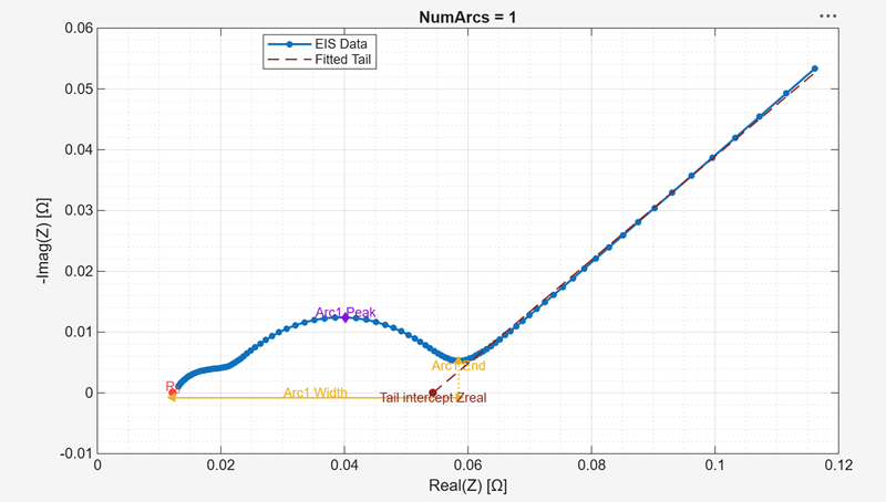
Nyquist plot that shows features for a single arc, with peak, width, and tail intercept

Assuming the same EIS data as the first example, extract features from by detecting two semicircular arcs. With a NumArcs setting of 2, the function separates the overlapping arcs and reports individual arc features. Compare the results with the single-arc extraction to observe how NumArcs affects the detected arc boundaries.

features = batteryEISFeatures(Zreal, Zimg, frequency, NumArcs=2, Plot=true);
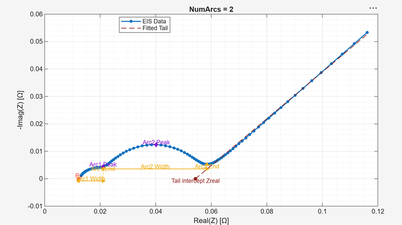
Nyquist plot that shows features for two arcs

Extract global features only (R0 and tail properties) when there are no arcs present in the Nyquist plot.

features = batteryEISFeatures(Zreal, Zimg, frequency, NumArcs=0);

Input Arguments

collapse all

Real part of the impedance, specified as a nonempty nonnegative double row vector. Zreal must be the same size as Zimg and F.

Imaginary part of the impedance, specified as a nonempty double row vector. Zimg must be the same size as Zreal and F. The function automatically handles sign conventions by standardizing to positive imaginary values (upper half-plane).

Frequency values in Hz, specified as a nonempty positive double row vector with unique values. frquency must be the same size as Zreal and Zimg.

Name-Value Arguments

collapse all

Specify optional pairs of arguments as Name1=Value1,...,NameN=ValueN, where Name is the argument name and Value is the corresponding value. Name-value arguments must appear after other arguments, but the order of the pairs does not matter.

Example: batteryEISFeatures(Zreal,Zimag,NumArcs=2) results in the detection of two semicircular arcs in the Nyquist plot.

Number of semicircular arcs to detect in the Nyquist plot, specified as 0, 1, or 2.

  • Set NumArcs to 0 to extract only global features such as R0 and tail properties. Use this value when there are no arcs present in the Nyquist plot.

  • Set NumArcs to 1 to extract one arc and global features. If there is more than one arc in the battery data, the function treats the overlapping arcs as a single combined arc.

  • Set NumArcs to 2 to extract two arcs and global features. If the function detects fewer arcs than NumArcs specifies, it issues a warning.

Display a Nyquist plot visualization of the extracted features, specified as a logical scalar. When set to true, the function creates a plot showing the original EIS data with annotated arcs, peaks, tail line, and R0.

Size of the smoothing window, specified as a positive integer.

If you do not specify this argument, the software determines the adaptive smoothing window size based on the data density, that is, the number of points with positive imaginary values.

  • Number of points < 50 — SmoothingWindowSize = 5

  • Otherwise — SmoothingWindowSize = 7

Output Arguments

collapse all

Extracted EIS features, returned as a table with one row. The following reference tables describe the contents of featureTable.

  • featureTable always contains the global features.

  • When NumArcs is greater than 0, featureTable also contains arc-specific features for each detected arc k.

Global FeaturesDescription

R0

High-frequency resistance in Ohms

R0_Frequency

Frequency at R0 in Hz

TailSlope

Slope of the linear tail region

TailIntercept_Zreal

X-intercept of the tail line in Ohms

Features for each Arc k (Arc1 shown)Description

Arc1_End_Zreal

Real impedance at arc end in Ohms

Arc1_End_Zimg

Imaginary impedance at arc end in Ohms

Arc1_Width

Arc width on the real axis in Ohms

Arc1_Peak_Zreal

Real impedance at arc peak in Ohms

Arc1_Peak_Zimg

Imaginary impedance at arc peak in Ohms

Arc1_Peak_Frequency

Frequency at arc peak in Hz

Arc1_End_Frequency

Frequency at arc end in Hz

Version History

Introduced in R2026b