Main Content

evaluateCGradient

Evaluate flux of PDE solution

Description

[cgradx,cgrady] = evaluateCGradient(results,xq,yq) returns the flux of PDE solution for the stationary equation at the 2-D points specified in xq and yq. The flux of the solution is the tensor product of c-coefficient and gradients of the PDE solution, cu.

example

[cgradx,cgrady,cgradz] = evaluateCGradient(results,xq,yq,zq) returns the flux of PDE solution for the stationary equation at the 3-D points specified in xq, yq, and zq.

example

[___] = evaluateCGradient(results,querypoints) returns the flux of PDE solution for the stationary equation at the 2-D or 3-D points specified in querypoints.

example

[___] = evaluateCGradient(___,iU) returns the flux of the solution of the PDE system for equation indices (components) iU. When evaluating flux for a system of PDEs, specify iU after the input arguments in any of the previous syntaxes.

The first dimension of cgradx, cgrady, and, in the 3-D case, cgradz corresponds to query points. The second dimension corresponds to equation indices iU.

example

[___] = evaluateCGradient(___,iT) returns the flux of PDE solution for the time-dependent equation or system of time-dependent equations at times iT. When evaluating flux for a time-dependent PDE, specify iT after the input arguments in any of the previous syntaxes. For a system of time-dependent PDEs, specify both equation indices (components) iU and time indices iT.

The first dimension of cgradx, cgrady, and, in the 3-D case, cgradz corresponds to query points. For a single time-dependent PDE, the second dimension corresponds to time-steps iT. For a system of time-dependent PDEs, the second dimension corresponds to equation indices iU, and the third dimension corresponds to time-steps iT.

example

[cgradx,cgrady] = evaluateCGradient(results) returns the flux of PDE solution of a 2-D problem at the nodal points of the triangular mesh. The shape of output arrays, cgradx and cgrady, depends on the number of PDEs for which results is the solution. The first dimension of cgradx and cgrady represents the node indices. For a system of stationary or time-dependent PDEs, the second dimension represents equation indices. For a single time-dependent PDE, the second dimension represents time-steps. The third dimension represents time-step indices for a system of time-dependent PDEs.

example

[cgradx,cgrady,cgradz] = evaluateCGradient(results) returns the flux of PDE solution of a 3-D problem at the nodal points of the tetrahedral mesh. The first dimension of cgradx, cgrady, and cgradz represents the node indices. The second dimension represents the equation indices. For a system of stationary or time-dependent PDEs, the second dimension represents equation indices. For a single time-dependent PDE, the second dimension represents time-steps. The third dimension represents time-step indices for a system of time-dependent PDEs.

example

Examples

collapse all

Solve the problem -Δu=1 on the L-shaped membrane with zero Dirichlet boundary conditions. Evaluate the tensor product of c-coefficient and gradients of the solution to a scalar elliptic problem at nodal and arbitrary locations. Plot the results.

Create a PDE model and geometry for this problem.

model = createpde;
geometryFromEdges(model,@lshapeg);
pdegplot(model,"FaceLabels","on")

Figure contains an axes object. The axes object contains 4 objects of type line, text.

Specify boundary conditions and coefficients.

applyBoundaryCondition(model,"dirichlet", ...
                             "Edge",1:model.Geometry.NumEdges, ...
                             "u",0);

specifyCoefficients(model,"m",0,"d",0,"c",10, ...
                          "a",0,"f",1,"Face",1);
specifyCoefficients(model,"m",0,"d",0,"c",5, ...
                          "a",0,"f",1,"Face",2);
specifyCoefficients(model,"m",0,"d",0,"c",1, ...
                          "a",0,"f",1,"Face",3);

Mesh the geometry and solve the problem.

generateMesh(model,"Hmax",0.05);
results = solvepde(model);
u = results.NodalSolution;

Compute the flux of the solution and plot the results.

[cgradx,cgrady] = evaluateCGradient(results);

figure
pdeplot(model,"XYData",u,"Contour","on","FlowData",[cgradx,cgrady])

Figure contains an axes object. The axes object contains 13 objects of type patch, line, quiver.

Compute the flux of the solution on the grid from -1 to 1 in each direction using the query points matrix.

v = linspace(-1,1,37);
[X,Y] = meshgrid(v);
querypoints = [X(:),Y(:)]';

[cgradxq,cgradyq] = evaluateCGradient(results,querypoints);

Alternatively, you can specify the query points as X,Y instead of specifying them as a matrix.

[cgradxq,cgradyq] = evaluateCGradient(results,X,Y);

Plot the result using the quiver plotting function.

figure
quiver(X(:),Y(:),cgradxq,cgradyq)
xlabel("x")
ylabel("y")

Figure contains an axes object. The axes object with xlabel x, ylabel y contains an object of type quiver.

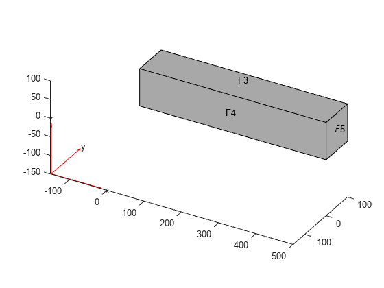
Compute stresses in a cantilever beam subject to shear loading at free end.

Create a PDE model and geometry for this problem.

N = 3;
model = createpde(N);
importGeometry(model,"SquareBeam.stl");
pdegplot(model,"FaceLabels","on")

Figure contains an axes object. The axes object contains 6 objects of type quiver, text, patch, line.

Specify coefficients and apply boundary conditions.

E = 2.1e11;
nu = 0.3;
c = elasticityC3D(E, nu);
a = 0;
f = [0;0;0];
specifyCoefficients(model,"m",0,"d",0,"c",c, ...
                          "a",a,"f",f);

applyBoundaryCondition(model,"dirichlet", ...
                             "Face",6, ...
                             "u",[0 0 0]);
applyBoundaryCondition(model,"neumann", ...
                             "Face",5, ...
                             "g",[0,0,-3e3]);

Mesh the geometry and solve the problem.

generateMesh(model,"Hmax",25,"GeometricOrder","quadratic");
results = solvepde(model);

Compute stress, that is, the product of c-coefficient and gradients of displacement.

[sig_xx,sig_yy,sig_zz] = evaluateCGradient(results);

Plot normal component of stress along x-direction. The top portion of the beam experiences tension, and the bottom portion experiences compression.

figure
pdeplot3D(model,"ColorMapData",sig_xx(:,1))

Figure contains an axes object. The hidden axes object contains 5 objects of type patch, quiver, text.

Define a line across the beam from the bottom to the top at mid-span and mid-width. Compute stresses along the line.

zg = linspace(0, 100, 10);
xg = 250*ones(size(zg));
yg = 50*ones(size(zg));

[sig_xx,sig_xy,sig_xz] = ...
evaluateCGradient(results,xg,yg,zg,1);

Plot the normal stress along x-direction.

figure
plot(sig_xx,zg)
grid on
xlabel("\sigma_{xx}")
ylabel("z")

Figure contains an axes object. The axes object with xlabel sigma indexOf xx baseline, ylabel z contains an object of type line.

Compute stresses in an idealized 3-D mechanical part under an applied load. First, create a PDE model for this problem.

N = 3;
model = createpde(N);

Import the geometry and plot it.

importGeometry(model,"BracketWithHole.stl");
figure
pdegplot(model,"FaceLabels","on")
view(30,30)
title("Bracket with Face Labels")

Figure contains an axes object. The axes object with title Bracket with Face Labels contains 6 objects of type quiver, text, patch, line.

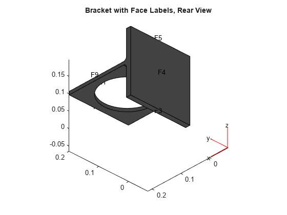
figure
pdegplot(model,"FaceLabels","on")
view(-134,-32)
title("Bracket with Face Labels, Rear View")

Figure contains an axes object. The axes object with title Bracket with Face Labels, Rear View contains 6 objects of type quiver, text, patch, line.

Specify coefficients and apply boundary conditions.

E = 200e9; % elastic modulus of steel in Pascals
nu = 0.3; % Poisson's ratio
c = elasticityC3D(E,nu);
a = 0;
f = [0;0;0]; % Assume all body forces are zero
specifyCoefficients(model,"m",0,"d",0,"c",c,"a",a,"f",f);

applyBoundaryCondition(model,"dirichlet","Face",4,"u",[0,0,0]);
distributedLoad = 1e4; % Applied load in Pascals
applyBoundaryCondition(model,"neumann","Face",8, ...
                             "g",[0,0,-distributedLoad]);

Mesh the geometry and solve the problem.

% Thickness of horizontal plate with hole, meters
bracketThickness = 1e-2;
% Maximum element length for a moderately fine mesh
hmax = bracketThickness;
generateMesh(model,"Hmax",hmax, ...
                   "GeometricOrder","quadratic");

result = solvepde(model);

Create a grid. For this grid, compute the stress tensor, which is the product of c-coefficient and gradients of displacement.

v = linspace(0,0.2,21);
[xq,yq,zq] = meshgrid(v);

[cgradx,cgrady,cgradz] = evaluateCGradient(result);

Extract individual components of stresses.

sxx = cgradx(:,1);
sxy = cgradx(:,2);
sxz = cgradx(:,3);

syx = cgrady(:,1);
syy = cgrady(:,2);
syz = cgrady(:,3);

szx = cgradz(:,1);
szy = cgradz(:,2);
szz = cgradz(:,3);

Compute von Mises stress.

sVonMises = sqrt( 0.5*( (sxx-syy).^2 + (syy -szz).^2 +...
           (szz-sxx).^2) + 3*(sxy.^2 + syz.^2 + szx.^2));

Plot von Mises stress. The maximum stress occurs at the weakest section. This section has the least material to support the applied load.

pdeplot3D(model,"ColorMapData",sVonMises)

Figure contains an axes object. The hidden axes object contains 5 objects of type patch, quiver, text.

Solve a 2-D transient heat transfer problem on a square domain and compute heat flow across convective boundary.

Create a PDE model for this problem.

model = createpde;

Create the geometry.

g = @squareg;
geometryFromEdges(model,g);
pdegplot(model,"EdgeLabels","on")
xlim([-1.2,1.2])
ylim([-1.2,1.2])
axis equal

Figure contains an axes object. The axes object contains 5 objects of type line, text.

Specify material properties and ambient conditions.

rho = 7800;
cp = 500;
k = 100;
Text = 25;
hext = 5000;

Specify the coefficients. Apply insulated boundary conditions on three edges and the free convection boundary condition on the right edge.

specifyCoefficients(model,"m",0,"d",rho*cp,"c",k,"a",0,"f",0);

applyBoundaryCondition(model,"neumann", ...
                             "Edge",[1,3,4], ...
                             "q",0,"g",0);
applyBoundaryCondition(model,"neumann", ...
                             "Edge", 2, ...
                             "q",hext,"g",Text*hext);

Set the initial conditions: uniform room temperature across domain and higher temperature on the left edge.

setInitialConditions(model,25);
setInitialConditions(model,100,"Edge",4);

Generate a mesh and solve the problem using 0:1000:200000 as a vector of times.

generateMesh(model);
tlist = 0:1000:200000;
results = solvepde(model,tlist);

Define a line at convection boundary to compute heat flux across it.

yg = -1:0.1:1;
xg = ones(size(yg));

Evaluate the product of c coefficient and spatial gradients at (xg,yg).

[qx,qy] = evaluateCGradient(results,xg,yg,1:length(tlist));

Spatially integrate gradients to obtain heat flow for each time-step.

HeatFlowX(1:length(tlist)) = -trapz(yg,qx(:,1:length(tlist)));

Plot convective heat flow over time.

figure
plot(tlist,HeatFlowX)
title("Heat flow across convection boundary")
xlabel("Time")
ylabel("Heat flow")

Figure contains an axes object. The axes object with title Heat flow across convection boundary, xlabel Time, ylabel Heat flow contains an object of type line.

Solve the heat transfer problem for the following 2-D geometry consisting of a square and a diamond made of different materials. Compute the heat flux density and plot it as a vector field.

Create a PDE model for this problem.

numberOfPDE = 1;
model = createpde(numberOfPDE);

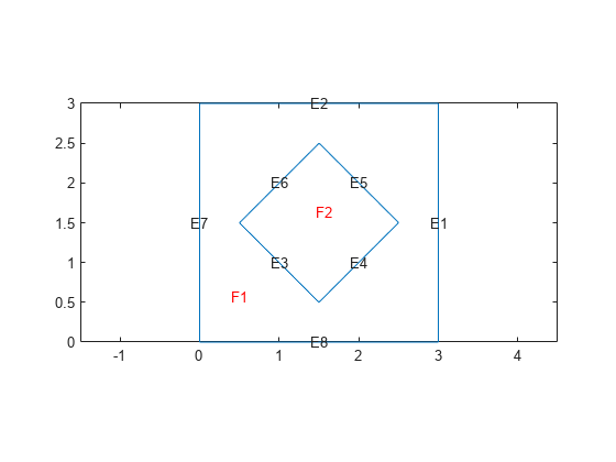
Create a geometry that consists of a square with an embedded diamond.

SQ1 = [3; 4; 0; 3; 3; 0; 0; 0; 3; 3];
D1 = [2; 4; 0.5; 1.5; 2.5; 1.5; 1.5; 0.5; 1.5; 2.5];
gd = [SQ1,D1];
sf = 'SQ1+D1';
ns = char('SQ1','D1');
ns = ns';
dl = decsg(gd,sf,ns);

geometryFromEdges(model,dl);

pdegplot(model,"EdgeLabels","on","FaceLabels","on")
xlim([-1.5,4.5])
ylim([-0.5,3.5])
axis equal

Figure contains an axes object. The axes object contains 11 objects of type line, text.

Set parameters for the square region.

rho_sq = 2;
C_sq = 0.1;
k_sq = 10;
Q_sq = 0;
h_sq = 0;

Set parameters for the diamond region.

rho_d = 1;
C_d = 0.1;
k_d = 2;
Q_d = 4;
h_d = 0;

Specify the coefficients for both subdomains. Apply the boundary and initial conditions.

specifyCoefficients(model,"m",0,"d",rho_sq*C_sq, ...
                          "c",k_sq,"a",h_sq, ...
                          "f",Q_sq,"Face",1);
specifyCoefficients(model,"m",0,"d",rho_d*C_d, ...
                          "c",k_d,"a",h_d, ...
                          "f",Q_d,"Face",2);

applyBoundaryCondition(model,"dirichlet", ...
                             "Edge",[1,2,7,8], ...
                             "h",1,"r",0);

setInitialConditions(model,0);

Mesh the geometry and solve the problem. To capture the most dynamic part of heat distribution process, solve the problem using logspace(-2,-1,10) as a vector of times.

generateMesh(model);

tlist = logspace(-2,-1,10);

results = solvepde(model,tlist);
u = results.NodalSolution;

Compute the heat flux density. Plot the solution with isothermal lines using a contour plot, and plot the heat flux vector field using arrows. The direction of the heat flow (from higher to lower temperatures) is opposite to the direction of cu. Therefore, use -cgradx and -cgrady to show the heat flow.

[cgradx,cgrady] = evaluateCGradient(results);

figure
pdeplot(model,"XYData",u(:,10),"Contour","on", ...
              "FlowData",[-cgradx(:,10),-cgrady(:,10)], ...
              "ColorMap","hot")

Figure contains an axes object. The axes object contains 13 objects of type patch, line, quiver.

Input Arguments

collapse all

PDE solution, specified as a StationaryResults object or a TimeDependentResults object. Create results using solvepde or createPDEResults.

Example: results = solvepde(model)

x-coordinate query points, specified as a real array. evaluateCGradient evaluates the tensor product of c-coefficient and gradients of the PDE solution at either the 2-D coordinate points [xq(i),yq(i)] or at the 3-D coordinate points [xq(i),yq(i),zq(i)]. So xq, yq, and (if present) zq must have the same number of entries.

evaluateCGradient converts query points to column vectors xq(:), yq(:), and (if present) zq(:). For a single stationary PDE, the result consists of column vectors of the same size. To ensure that the dimensions of the returned x-, y-, and z-components are consistent with the dimensions of the original query points, use reshape. For example, use cgradx = reshape(cgradx,size(xq)).

For a time-dependent PDE or a system of PDEs, the first dimension of the resulting arrays corresponds to spatial points specified by the column vectors xq(:), yq(:), and (if present) zq(:).

Data Types: double

y-coordinate query points, specified as a real array. evaluateCGradient evaluates the tensor product of c-coefficient and gradients of the PDE solution at either the 2-D coordinate points [xq(i),yq(i)] or at the 3-D coordinate points [xq(i),yq(i),zq(i)]. So xq, yq, and (if present) zq must have the same number of entries.

evaluateCGradient converts query points to column vectors xq(:), yq(:), and (if present) zq(:). For a single stationary PDE, the result consists of column vectors of the same size. To ensure that the dimensions of the returned x-, y-, and z-components are consistent with the dimensions of the original query points, use reshape. For example, use cgrady = reshape(cgrady,size(yq)).

For a time-dependent PDE or a system of PDEs, the first dimension of the resulting arrays corresponds to spatial points specified by the column vectors xq(:), yq(:), and (if present) zq(:).

Data Types: double

z-coordinate query points, specified as a real array. evaluateCGradient evaluates the tensor product of c-coefficient and gradients of the PDE solution at the 3-D coordinate points [xq(i),yq(i),zq(i)]. So xq, yq, and zq must have the same number of entries.

evaluateCGradient converts query points to column vectors xq(:), yq(:), and zq(:). For a single stationary PDE, the result consists of column vectors of the same size. To ensure that the dimensions of the returned x-, y-, and z-components are consistent with the dimensions of the original query points, use reshape. For example, use cgradz = reshape(cgradz,size(zq)).

For a time-dependent PDE or a system of PDEs, the first dimension of the resulting arrays corresponds to spatial points specified by the column vectors xq(:), yq(:), and (if present) zq(:).

Data Types: double

Query points, specified as a real matrix with either two rows for 2-D geometry or three rows for 3-D geometry. evaluateCGradient evaluates the tensor product of c-coefficient and gradients of the PDE solution at the coordinate points querypoints(:,i), so each column of querypoints contains exactly one 2-D or 3-D query point.

Example: For 2-D geometry, querypoints = [0.5,0.5,0.75,0.75; 1,2,0,0.5]

Data Types: double

Time indices, specified as a vector of positive integers. Each entry in iT specifies a time index.

Example: iT = 1:5:21 specifies every fifth time-step up to 21.

Data Types: double

Equation indices, specified as a vector of positive integers. Each entry in iU specifies an equation index.

Example: iU = [1,5] specifies the indices for the first and fifth equations.

Data Types: double

Output Arguments

collapse all

x-component of the flux of the PDE solution, returned as an array. The first array dimension represents the node index. If results is a StationaryResults object, the second array dimension represents the equation index for a system of PDEs. If results is a TimeDependentResults object, the second array dimension represents either the time-step for a single PDE or the equation index for a system of PDEs. The third array dimension represents the time-step index for a system of time-dependent PDEs. For information about the size of cgradx, see Dimensions of Solutions, Gradients, and Fluxes.

For query points that are outside the geometry, cgradx = NaN.

y-component of the flux of the PDE solution, returned as an array. The first array dimension represents the node index. If results is a StationaryResults object, the second array dimension represents the equation index for a system of PDEs. If results is a TimeDependentResults object, the second array dimension represents either the time-step for a single PDE or the equation index for a system of PDEs. The third array dimension represents the time-step index for a system of time-dependent PDEs. For information about the size of cgrady, see Dimensions of Solutions, Gradients, and Fluxes.

For query points that are outside the geometry, cgrady = NaN.

z-component of the flux of the PDE solution, returned as an array. The first array dimension represents the node index. If results is a StationaryResults object, the second array dimension represents the equation index for a system of PDEs. If results is a TimeDependentResults object, the second array dimension represents either the time-step for a single PDE or the equation index for a system of PDEs. The third array dimension represents the time-step index for a system of time-dependent PDEs. For information about the size of cgradz, see Dimensions of Solutions, Gradients, and Fluxes.

For query points that are outside the geometry, cgradz = NaN.

Tips

  • While the results object contains the solution and its gradient (both calculated at the nodal points of the triangular or tetrahedral mesh), it does not contain the flux of the PDE solution. To compute the flux at the nodal locations, call evaluateCGradient without specifying locations. By default, evaluateCGradient uses nodal locations.

Version History

Introduced in R2016b