ModalThermalResults
Description
A ModalThermalResults object contains the eigenvalues and
eigenvector matrix of a thermal analysis problem, and average of snapshots used for proper
orthogonal decomposition (POD).
Creation
Solve a modal thermal problem using the solve function. This function returns a modal thermal solution as a ModalThermalResults object.
Properties
This property is read-only.
Eigenvalues of a thermal problem, returned as a column vector.
Data Types: double
This property is read-only.
Eigenvector matrix, returned as a matrix.
Data Types: double
This property is read-only.
Average of snapshots used for POD, returned as a column vector.
Data Types: double
This property is read-only.
Type of modes, returned as "EigenModes" or
"PODModes".
Data Types: string
This property is read-only.
Finite element mesh, returned as an FEMesh object.
Examples
Solve a transient thermal problem by first obtaining mode shapes for a particular decay range and then using the modal superposition method.
Modal Decomposition
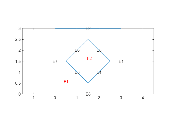
Create a geometry representing a square plate with a diamond-shaped region in its center.
SQ1 = [3; 4; 0; 3; 3; 0; 0; 0; 3; 3];
D1 = [2; 4; 0.5; 1.5; 2.5; 1.5; 1.5; 0.5; 1.5; 2.5];
gd = [SQ1 D1];
sf = 'SQ1+D1';
ns = char('SQ1','D1');
ns = ns';
g = decsg(gd,sf,ns);
pdegplot(g,EdgeLabels="on",FaceLabels="on")
xlim([-1.5 4.5])
ylim([-0.5 3.5])
axis equal

Create an femodel object for modal thermal analysis and include the geometry.
model = femodel(AnalysisType="thermalModal", ...
                Geometry=g);
For the square region, assign these thermal properties:
Thermal conductivity is .
Mass density is .
Specific heat is .
model.MaterialProperties(1) = ...
    materialProperties(ThermalConductivity=10, ...
                       MassDensity=2, ...
                       SpecificHeat=0.1);
For the diamond region, assign these thermal properties:
Thermal conductivity is .
Mass density is .
Specific heat is .
model.MaterialProperties(2) = ...
    materialProperties(ThermalConductivity=2, ...
                       MassDensity=1, ...
                       SpecificHeat=0.1);
Assume that the diamond-shaped region is a heat source with a density of .
model.FaceLoad(2) = faceLoad(Heat=4);
Apply a constant temperature of 0 °C to the sides of the square plate.
model.EdgeBC(1:4) = edgeBC(Temperature=0);
Set the initial temperature to 0 °C.
model.FaceIC = faceIC(Temperature=0);
Generate the mesh.
model = generateMesh(model);
Compute eigenmodes of the model in the decay range [100,10000] .
RModal = solve(model,DecayRange=[100,10000])
RModal =
  ModalThermalResults with properties:

    DecayRates: [164×1 double]
    ModeShapes: [1461×164 double]
      ModeType: "EigenModes"
          Mesh: [1×1 FEMesh]
Transient Analysis
Knowing the mode shapes, you can now use the modal superposition method to solve the transient thermal problem. First, switch the model analysis type to thermal transient.
model.AnalysisType = "thermalTransient";The dynamics for this problem are very fast. The temperature reaches a steady state in about 0.1 second. To capture the most active part of the dynamics, set the solution time to logspace(-2,-1,100). This command returns 100 logarithmically spaced solution times between 0.01 and 0.1.
tlist = logspace(-2,-1,10);
Solve the equation.
Rtransient = solve(model,tlist,ModalResults=RModal);
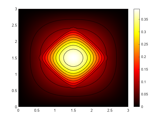
Plot the solution with isothermal lines by using a contour plot.
msh = Rtransient.Mesh
msh =
  FEMesh with properties:

             Nodes: [2×1461 double]
          Elements: [6×694 double]
    MaxElementSize: 0.1697
    MinElementSize: 0.0849
     MeshGradation: 1.5000
    GeometricOrder: 'quadratic'
T = Rtransient.Temperature;
pdeplot(msh,XYData=T(:,end),Contour="on", ...
                            ColorMap="hot")
axis equal

Obtain POD modes of a linear thermal problem using several instances of the transient solution (snapshots).
Create an femodel object for transient thermal analysis and include a unit square geometry in the model.
model = femodel(AnalysisType="thermalTransient", ...
                Geometry=@squareg);
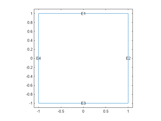
Plot the geometry, displaying edge labels.
pdegplot(model.Geometry,EdgeLabels="on")
xlim([-1.1 1.1])
ylim([-1.1 1.1])
Specify the thermal conductivity, mass density, and specific heat of the material.
model.MaterialProperties = ...
    materialProperties(ThermalConductivity=400, ...
                       MassDensity=1300, ...
                       SpecificHeat=600);
Set the temperature on the right edge to 100.
model.EdgeBC(2) = edgeBC(Temperature=100);
Set an initial value of 0 for the temperature.
model.FaceIC = faceIC(Temperature=0);
Generate a mesh.
model = generateMesh(model);
Solve the model for three different values of heat source and collect snapshots.
tlist = 0:10:600;
snapShotIDs = [1:10 59 60 61];
Tmatrix = [];

heatVariation = [10000 15000 20000];
for q = heatVariation
    model.FaceLoad = faceLoad(Heat=q);
    results = solve(model,tlist);
    Tmatrix = [Tmatrix,results.Temperature(:,snapShotIDs)];
end
Switch the model analysis type to thermal modal.
model.AnalysisType = "thermalModal";Compute the POD modes.
RModal = solve(model,Snapshots=Tmatrix)
RModal =
  ModalThermalResults with properties:

          DecayRates: [6×1 double]
          ModeShapes: [1529×6 double]
    SnapshotsAverage: [1529×1 double]
            ModeType: "PODModes"
                Mesh: [1×1 FEMesh]
Version History
Introduced in R2022a
See Also
Functions
Objects
MATLAB Command
You clicked a link that corresponds to this MATLAB command:
Run the command by entering it in the MATLAB Command Window. Web browsers do not support MATLAB commands.
Select a Web Site
Choose a web site to get translated content where available and see local events and offers. Based on your location, we recommend that you select: .
You can also select a web site from the following list
How to Get Best Site Performance
Select the China site (in Chinese or English) for best site performance. Other MathWorks country sites are not optimized for visits from your location.
Americas
- América Latina (Español)
- Canada (English)
- United States (English)
Europe
- Belgium (English)
- Denmark (English)
- Deutschland (Deutsch)
- España (Español)
- Finland (English)
- France (Français)
- Ireland (English)
- Italia (Italiano)
- Luxembourg (English)
- Netherlands (English)
- Norway (English)
- Österreich (Deutsch)
- Portugal (English)
- Sweden (English)
- Switzerland
- United Kingdom (English)