Simulate GNSS Multipath Effects in Urban Canyon Environment

This example shows how to simulate Global Navigation Satellite System (GNSS) or Global Positioning System (GPS) receiver noises due to local obstructions in the environment of the receiver.

A GNSS receiver estimates the current position from information obtained from satellites in view. When a receiver is in a location with many local obstructions, it can suffer from multipath. Multipath is when the satellite signals arrive at the receiver antenna from two or more paths. One or none of these paths is a direct line-of-sight (LOS) from the satellite to the receiver. The remainder of the paths contain reflections from the local obstructions. Each satellite signal contains a transmission timestamp that you can use in addition to the receiver clock to compute a pseudorange between the satellite and the receiver. A satellite signal arriving by a nondirect path results in an incorrect pseudorange that is larger than the pseudorange from a direct path. The incorrect pseudoranges degrade the accuracy of the estimated receiver position.

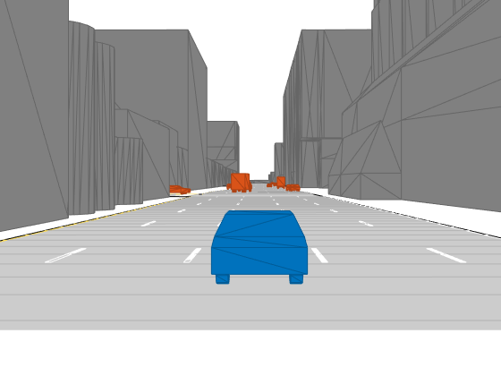
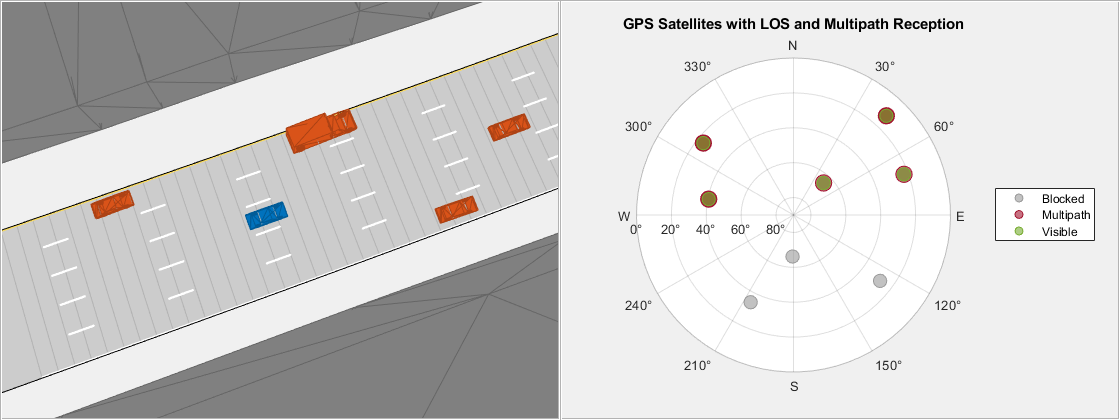
This image shows a car driving on a street in a driving scenario in downtown Boston, MA, with tall buildings on either side of the street. As the car drives, you can see a skyplot on the right that shows the satellites in view of the receiver.

Load Driving Scenario

Load a MAT file containing a drivingScenario object created from an OSM file of downtown Boston, MA. The OSM file was downloaded from https://www.openstreetmap.org, which provides access to crowdsourced map data all over the world. The data is licensed under the Open Data Commons Open Database License (ODbL), https://opendatacommons.org/licenses/odbl/.

The scenario contains an urban environment similar to a canyon, with tall buildings on both sides of the vehicle.

load("downtownBostonDrivingScenario.mat","scenario","egoVehicle")
fig = figure;
ax = axes(fig);
chasePlot(egoVehicle,Meshes="on",Parent=ax)

Create GNSS Receiver Sensor Model

Set the RNG seed to produce the same results when executing the example multiple times. Create a gnssMeasurementGenerator object and set the sample rate and reference location by specifying the SampleTime and GeoReference properties of the drivingScenario object, respectively. Set the initial time of the gnssMeasurementGenerator object to August 12, 2022, at 10 AM.

rng default
t0 = datetime(2022,12,8,10,0,0);
gnss = gnssMeasurementGenerator(SampleRate=1/scenario.SampleTime, ...
                                ReferenceLocation=scenario.GeoReference, ...
                                InitialTime=t0);

Attach the gnssMeasurementGenerator object to the ego Vehicle of the scenario with the mounting location set to 1.5 meters along the z-axis from the origin of the car.

mountingLocation = [0 0 1.5];
addSensors(scenario,{gnss},egoVehicle.ActorID,mountingLocation);

Run Scenario and Visualize Multipath

Set up a chase plot and sky plot to visualize the scenario by using chaseplot and skyplot, respectively. The chase plot shows the car, egoVehicle, from above to show the local obstructions that interfere with the GPS satellite signals. The sky plot shows all the GPS satellites currently in view of the ego vehicle as the car moves. Depending on visibility, each satellite is in one of these categories:

• Blocked — The GPS receiver detects no signal from the satellite.

• Multipath — The GPS receiver detects signals from the satellite, but with one or more reflections.

• Visible — The GPS receiver detects a signal and has direct line-of-sight (LOS) with the satellite.

Note that multiple signals from the same satellite can be found.

Resize the figure to fit both plots.

clf(fig,"reset")
set(fig,Position=[400 458 1120 420])

Create a UI panel on the left side of the figure and create axes for a chase plot. Add the chase plot with the top of the plot as north and set the chase plot to follow the car viewed from above.

hChasePlot = uipanel(fig,Position=[0 0 0.5 1]);
ax = axes(hChasePlot);
viewYawAngle = 90-egoVehicle.Yaw; % Make the top of the plot point north.
chasePlot(egoVehicle,Parent=ax,Meshes="on",ViewHeight=75, ...
          ViewPitch=80,ViewYaw=viewYawAngle,ViewLocation=[0 -2.5*egoVehicle.Length]);

Create a UI panel on the right side of the figure and create axes for a sky plot to show the satellite visibility. Add an empty sky plot to the panel. Set the color order to gray, red, and green representing blocked, multipath, and visible satellite statuses, respectively.

hSkyPlot = uipanel(fig,Position=[0.5 0 0.5 1]);
sp = skyplot(NaN,NaN,Parent=hSkyPlot);
title("GPS Satellites with LOS and Multipath Reception");
legend(sp)
colors = colororder(sp);
colororder(sp,[0.6*[1 1 1];colors(7,:);colors(5,:)]);

Run the driving scenario. At each step of the scenario:

1. Read satellite pseudoranges.

2. Get satellite azimuths and elevations from satellite positions.

3. Categorize the satellites based on their status (Blocked, Multipath, or Visible).

4. Set different marker sizes so that multiple measurements from the same satellite can be seen.

5. Update the sky plot.

currTime = gnss.InitialTime;
while advance(scenario)
    % Read satellite pseudoranges.
    [p,satPos,status] = gnss();
    allSatPos = gnssconstellation(currTime);
    currTime = currTime + seconds(1/gnss.SampleRate);
    
    % Get satellite azimuths and elevations from satellite positions.
    trueRecPos = enu2lla(egoVehicle.Position,gnss.ReferenceLocation,"ellipsoid");
    [az, el] = lookangles(trueRecPos,satPos,gnss.MaskAngle);
    [allAz,allEl,vis] = lookangles(trueRecPos,allSatPos,gnss.MaskAngle);
    allEl(allEl<0) = NaN;
    
    % Set categories of satellites based on the status (Blocked, Multipath, or Visible).
    groups = categorical([-ones(size(allAz)); status.LOS],[-1 0 1],["Blocked","Multipath","Visible"]); 
    
    % Set different marker sizes so that multiple measurements from the same satellite can be seen. 
    markerSizes = 100*ones(size(groups));
    markerSizes(groups == "Multipath") = 150;
    
    % Update the sky plot.
    set(sp,AzimuthData=[allAz; az],ElevationData=[allEl; el],GroupData=groups,MarkerSizeData=markerSizes);
    drawnow;
end

Conclusion

This example showed how to generate raw GNSS measurements affected by multipath propagation from local obstructions. You can use these measurements to estimate the position of the GPS receiver, or combined with other sensors, such as an inertial measurement unit (IMU), to improve the position estimation. See the Ground Vehicle Pose Estimation for Tightly Coupled IMU and GNSS example for more information. Determining if a raw GNSS measurement contains multipath propagation can be difficult. One detection technique is innovation or residual filtering. See the Detect Multipath GPS Reading Errors Using Residual Filtering in Inertial Sensor Fusion example for more information.