Model a Continuous-Time Delta Sigma Modulator With Inherent Anti-Aliasing Property

Open Live Script

This example shows how to design a Continuous-time Delta Sigma Modulator (CT DSM) using the DT-CT Translation method explained in [1]. CT DSMs can also be designed using Direct Synthesis of CT DSMs [2].

Continuous-time DSM

In a CT DSM, sampling happens after the loop filter which alleviates settling issues present in discrete-time loop filters especially at high speeds. Moreover, CT DSMs have inherent anti-aliasing property, i.e., the modulator also acts like an anti-alias filter.

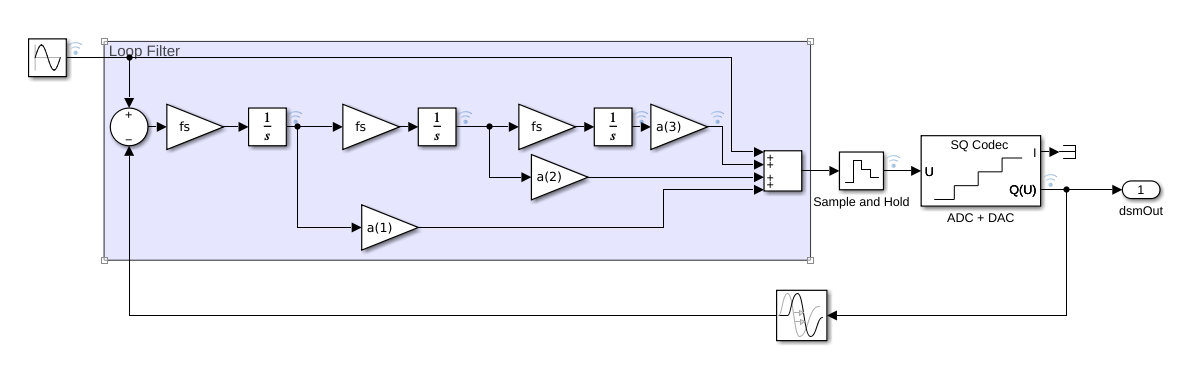
The block diagram of a third order CT DSM is shown below. Its loop filter operates in the continuous time domain and sampling is performed at the input of the ADC.

Noise Transfer Function Design

The first step in the CT DSM design is to obtain an NTF using the same methods used to obtain an NTF for DT DSMs. You can use the function called synthesizeNTF() from Delta-Sigma Toolbox [3] to obtain the desired NTF. The next step is to obtain the coefficients of a CT filter using impulse-invariance method. Detailed explanation of these steps can be found in [1]. These steps are implemented in the function dsmAdcFindCTcoeff(). You will use it to model a feed-forward CT DSM and a feedback CT DSM.

Feed-forward CT DSM

In this section you will design a third order feed-forward CT DSM as explained in [1]. The modulator employs a 4-bit quantizer resulting in 16 levels, an oversampling ratio of 64 and a sampling frequency of 128 kHz, resulting in a bandwidth of 1 kHz. Use the function dsmAdcFindCTcoeff() to generate the CT filter gain coefficients.

order = 3; % Modulator order
OSR = 64; %Oversampling ratio 
form = 'FF'; % Feedforward modulator
fs = 128e3; %Sampling frequency (Hz)
optimFlag = 0; % optimization option for synthesizeNTF()
Hinf = 2.5; %Infinity norm 
f0 = 0; % low-pass modulator

[aff, gff, bff, cff] = msblks.ADC.dsmAdcFindCTcoeff(order, OSR, form, optimFlag, Hinf, f0);

Open the model and set the relative tolerance parameter RelTol to 1e-6 to increase simulation accuracy.

model = 'ct3rdOrderFF';
open(model);
set_param(model, 'RelTol', '1e-6');

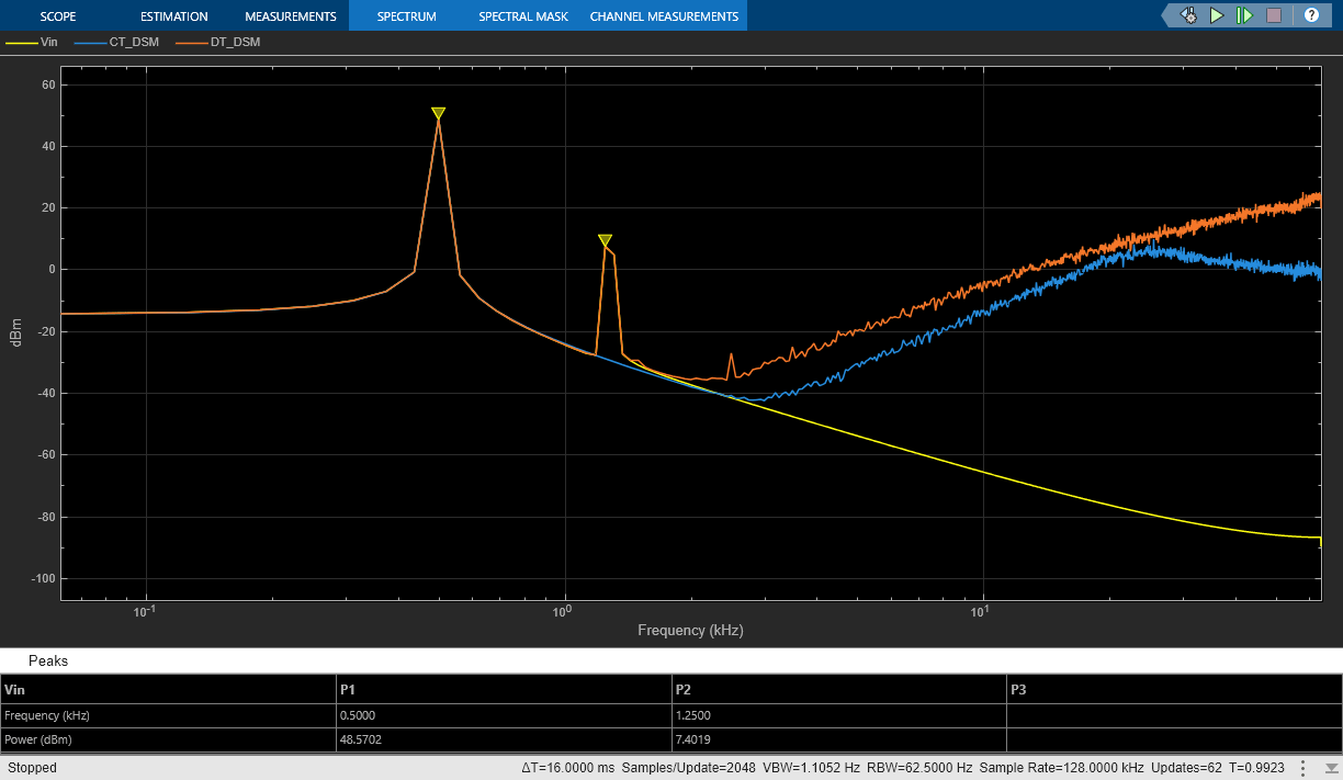
For performance comparison, the model also employs a third order Discrete Time (DT) DSM which uses the same NTF as the one used for DT-CT transformation. The input stimulus comprises two sinusoids - one at 500 Hz and another at 99% of the sampling frequency.

Run the simulation and observe that there is no aliased signal in the output of CT DSM whereas the aliased signal of the second sinusoid is present in the output of DT DSM.

out=sim(model);

You can also estimate the SNR and ENOB from the output of the two DSMs using the function dsmAdcEstimateSNR().

[SNR_CT_ff, ENOB_CT_ff] = msblks.ADC.dsmAdcEstimateSNR(out.ctdsmoutff', OSR)

SNR_CT_ff = 114.1513

ENOB_CT_ff = 18.6696

[SNR_DT_ff, ENOB_DT_ff] = msblks.ADC.dsmAdcEstimateSNR(out.dtdsmoutff', OSR)

SNR_DT_ff = 102.1897

ENOB_DT_ff = 16.6827

Feedback CT DSM

In this section, you will design a third order feedback CT DSM using the same parameters as in the previous section.

order = 3; % Modulator order
OSR = 64; %Oversampling ratio
form = 'FB'; %Feedback modulator
fs = 128e3; %Sampling frequency (Hz)
optimFlag = 0; % optimization option for synthesizeNTF()
Hinf = 2.5; %Infinity norm
f0 = 0; % low-pass modulator

[a, g, b, c] = msblks.ADC.dsmAdcFindCTcoeff(order, OSR, form, optimFlag, Hinf, f0);

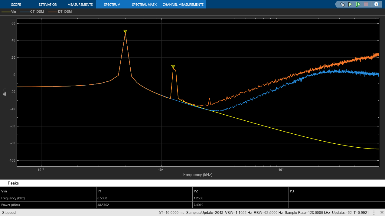
Open the model and simulate. The performance of the feedback modulator is similar to that of the feed-forward modulator including the anti-aliasing behavior.

model = "ct3rdOrderFB";
open(model);
set_param(model, 'RelTol', '1e-6');
out=sim(model);

[SNR_CT_fb, ENOB_CT_fb] = msblks.ADC.dsmAdcEstimateSNR(out.ctdsmoutfb', OSR)

SNR_CT_fb = 114.2185

ENOB_CT_fb = 18.6808

[SNR_DT_fb, ENOB_DT_fb] = msblks.ADC.dsmAdcEstimateSNR(out.dtdsmoutfb', OSR)

SNR_DT_fb = 102.1972

ENOB_DT_fb = 16.6839

Conclusion

You have modeled a feed-forward CT DSM using the principles explained in [1]. You were also able to verify that the same principles can be used to design a feedback CT DSM. You also saw that the CT DSMs can double down as anti-aliasing filters.

References

[3] Richard Schreier (2022). Delta Sigma Toolbox (https://www.mathworks.com/matlabcentral/fileexchange/19-delta-sigma-toolbox), MATLAB Central File Exchange. Retrieved June 14, 2022.

References

[1] Shanthi Pavan; Richard Schreier; Gabor C. Temes, Understanding Delta-Sigma Data Converters, second edition, IEEE Press, copyright 2017.
[2] Jose M. de la Rosa, Sigma-Delta Converters, second edition, copyright 2018.