Surge Tank Control Using Discrete Control Set MPC
This example shows how to use a linear MPC controller with both continuous- and discrete-set control actions to control the level of a surge tank in Simulink®.
Overview
Many petrochemical processes include surge capacity to insulate downstream operations from upsets in upstream flows. This example considers a liquid surge tank supplied by two pumps.
Pump 1 is variable-speed and can deliver a flow rate between 0 and 100 L/min. The rate of change of the flow rate is limited to 50 L/min per minute.
Pump 2 is on-off and delivers 100 L/min when it is on.
This system also has a continuously adjustable valve that regulates the tank discharge to accommodate a downstream process.
mdl = 'ReservoirMPC';
open_system(mdl)
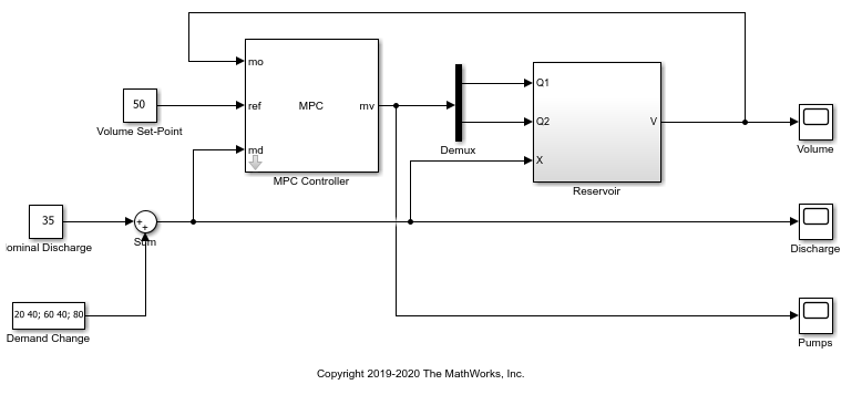
The control objective is to use the two pumps (manipulated variables) to maintain the tank volume at its setpoint when the discharge valve introduces a disturbance to the surge tank (measured disturbance).
When downstream demand is constant, pump 1 controls the surge tank level, ideally keeping it near 50%. When a disturbance occurs, both pumps can go into action to maintain the tank volume between 25% and 75% during the transient time. When downstream demand is high, however, Pump 2 must turn on.
In summary, the MPC controller manages the two pumps such that:
The tank level stays near 50% when demand is constant.
The tank level stays within the ideal range when Pump 2 turns on and off. Rapid Pump 2 on-off cycling is undesirable.
Create Linear Plant from Nonlinear Surge Tank Model
In the Simulink model, the surge tank model is in the Reservoir subsystem. It implements the following equations.
dV/dt = Qin - Qout, whereVis the tank volume between 0 and 100 (percent)Qin = Q1 + Q2, the sum of the two pump flow rates (L/min)Qout = 0.2*sqrt(2)*X*sqrt(V), the discharge rate (L/min)X, the discharge valve, which can open between 0 and 100 (percent)
The plant starts running at its nominal steady-state operating point: pump 1 runs at 70 L/min, pump 2 is off, the discharge valve is at 35%, and the tank volume is at 50%. Create a linear model of the tank at this operating point. This model has three inputs: the manipulated variables Q1 and Q2, and the measured disturbance|X|.
plant = ss(-0.7,[1 1 -2],1,[0 0 0]);
plant = setmpcsignals(plant,'MV',[1 2],'MD',3);
Design MPC Controller with Continuous and Discrete Control Actions
Create a linear MPC controller with a sample time of one second, default prediction and control horizons, and default cost function weights.
Ts = 1;
mpcobj = mpc(plant,Ts);
-->"PredictionHorizon" is empty. Assuming default 10.
-->"ControlHorizon" is empty. Assuming default 2.
-->"Weights.ManipulatedVariables" is empty. Assuming default 0.00000.
-->"Weights.ManipulatedVariablesRate" is empty. Assuming default 0.10000.
-->"Weights.OutputVariables" is empty. Assuming default 1.00000.
Set the nominal values for the controller to match the steady-state operating point.
mpcobj.Model.Nominal.U = [70; 0; 35];
mpcobj.Model.Nominal.Y = 50;
mpcobj.Model.Nominal.X = 50;
mpcobj.Model.Nominal.DX = 0;
Choose the MVRate weights such that the controller adjusts pump 1 in preference to pump 2. That is, the controller penalizes pump 2 adjustments less than pump 1 adjustments.
mpcobj.Weights.MVrate = [0.1 0.2];
Specify safety bounds on the continuous input and output signals.
mpcobj.OV.Min = 0;
mpcobj.OV.Max = 100;
mpcobj.MV(1).Min = 0;
mpcobj.MV(1).Max = 100;
mpcobj.MV(1).RateMin = -50;
mpcobj.MV(1).RateMax = 50;
Because pump 2 has two discrete settings (0 and 100 L/min), specify a discrete set in the Type property of this controller. Depending on your application, the Type property can also be binary or integer.
mpcobj.MV(2).Type = [0 100];
Simulate Closed-Loop Response with Discharge Disturbance
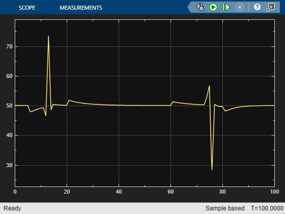
The simulation begins at the nominal condition. At t = 5, the discharge rate ramps up until pump 1 is at its full capacity and pump 2 must turn on. Pump 2 turns on at t = 12. Pump 1 must then decrease as rapidly as possible to keep the level in bounds, then establish a new steady-state operating point. At t = 60, the discharge begins to ramp down to the nominal state. The MPC controller keeps the volume within the ideal range, and pump 2 does not exhibit rapid cycling.
sim(mdl)
open_system([mdl '/Volume'])
-->Converting model to discrete time.
-->Integrator added as output disturbance model for measured output #1.
-->"Model.Noise" is empty. Assuming white noise on each measured output.

ans =

  Simulink.SimulationOutput:
                   tout: [106x1 double]

     SimulationMetadata: [1x1 Simulink.SimulationMetadata]
           ErrorMessage: [0x0 char]
The following figure shows the flow rates from two pumps.
open_system([mdl '/Pumps'])
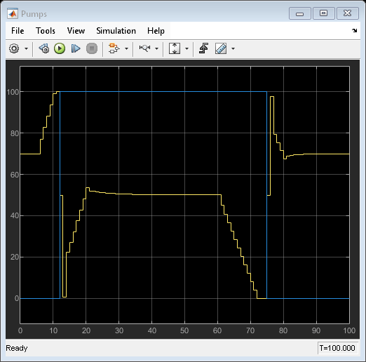
As expected, the MPC controller turns pump 2 on and off.
bdclose(mdl) % close simulink model.