Control Robot Manipulator Using Passivity-Based Nonlinear MPC
This example shows how to design a passivity-based controller for a robot manipulator using nonlinear model predictive control (MPC).
Overview
The dynamics for a two-link robot manipulator can be written as follows [1].
Here, , , and are 2-by-1 vectors that represent the joint angles, velocities, and accelerations. The control input vector is the torque .
is the manipulator inertia matrix.
is the Coriolis matrix.
is the gravity vector.
These robot dynamics are implemented in manipulatorStateFcn.m.
The control objective is to select torque such that the joint angles track a desired reference . To enforce closed-loop stability, the controller includes a passivity constraint [2].
Passivity Constraint
To define the passivity constraint, first define the tracking error vector as the difference between the joint angles and the desired reference angles.
To achieve good tracking performance, define the storage function as , where . Take the derivative of to obtain the relationship , where
.
Therefore, the system is passive from to . The relationship between the passivity input and torque is described in the helper function getPassivityInput.m.
To enforce closed-loop stability, define the passivity constraint as follows [2].
with .
For a nonlinear MPC controller, you define the passivity constraint by setting the Passivity property of the nonlinear MPC object.
Design Nonlinear MPC Controller
Create a nonlinear MPC object with four states, four outputs, and two inputs.
nlobj = nlmpc(4,4,2);
Zero weights are applied to one or more OVs because there are fewer MVs than OVs.
Specify the prediction model state function using the robot dynamics function.
nlobj.Model.StateFcn = "manipulatorStateFcn";Specify a sample time of 0.1 seconds and use default prediction and control horizons.
nlobj.Ts = 0.1;
The default cost function in nonlinear MPC is a standard quadratic cost function, which is suitable for reference tracking. In this example, the goal is to have the first two states follow a given reference trajectory. Therefore, specify nonzero tuning weights for the first two output variables.
nlobj.Weights.OutputVariables = [2 1 0 0];
nlobj.Weights.ManipulatedVariablesRate = [0 0];
Specify the fields of the passivity property of the nonlinear MPC object.
nlobj.Passivity.EnforceConstraint = true;
nlobj.Passivity.InputFcn = "getPassivityInput";
nlobj.Passivity.OutputFcn = "getPassivityOutput";
Closed-Loop Simulation
Specify the initial conditions of the states.
x0 = [-2;-1;1;1];
Open the Simulink® model.
mdl = "manipulatorNLMPC";
open_system(mdl)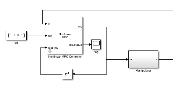
Run the model.
sim(mdl);
View the manipulator states. Both joint angles reach and stay at the target value of 1.
open_system(mdl + "/Manipulator/states")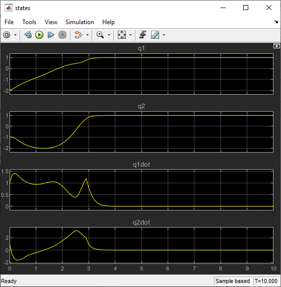
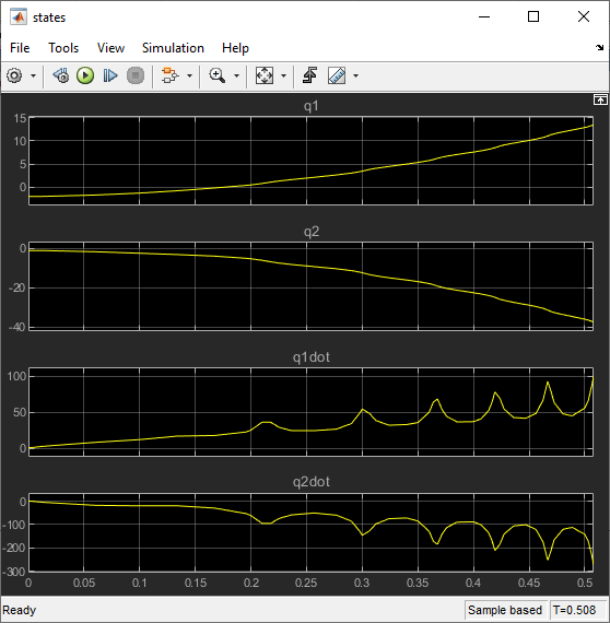
To view the performance of the nonlinear MPC controller without the passivity constraint, remove it from the controller.
nlobj.Passivity.EnforceConstraint = false;
Run the simulation.
sim(mdl);

Without the passivity constraint, the closed-loop system becomes unstable with the same controller design parameters.

References
[1] Hatanaka, Takeshi, Nikhil Chopra, Masayuki Fujita, and Mark W. Spong. Passivity-Based Control and Estimation in Networked Robotics. Communications and Control Engineering. Cham: Springer International Publishing, 2015. https://doi.org/10.1007/978-3-319-15171-7.
[2] Raff, Tobias, Christian Ebenbauer, and Frank Allgöwer. “Nonlinear Model Predictive Control: A Passivity-Based Approach.” In Assessment and Future Directions of Nonlinear Model Predictive Control, edited by Rolf Findeisen, Frank Allgöwer, and Lorenz T. Biegler, 358:151–62. Berlin, Heidelberg: Springer Berlin Heidelberg, 2007. https://doi.org/10.1007/978-3-540-72699-9_12.