About Passivity and Passivity Indices

Passive control is often part of the safety requirements in applications such as process control, tele-operation, human-machine interfaces, and system networks. A system is passive if it cannot produce energy on its own, and can only dissipate the energy that is stored in it initially. More generally, an I/O map is passive if, on average, increasing the output y requires increasing the input u.

For example, a PID controller is passive because the control signal (the output) moves in the same direction as the error signal (the input). But a PID controller with delay is not passive, because the control signal can move in the opposite direction from the error, a potential cause of instability.

Most physical systems are passive. The Passivity Theorem holds that the negative-feedback interconnection of two strictly passive systems is passive and stable. As a result, it can be desirable to enforce passivity of the controller for a passive system, or to passivate the operator of a passive system, such as the driver of a car.

In practice, passivity can easily be destroyed by the phase lags introduced by sensors, actuators, and communication delays. These problems have led to extension of the Passivity Theorem that consider excesses or shortages of passivity, frequency-dependent measures of passivity, and a mix of passivity and small-gain properties.

Passive Systems

A linear system $$G(s)$$ is passive if all input/output trajectories $$y(t)=Gu(t)$$ satisfy:

$${\int }_0^T{y}^T(t)u(t)dt>0,\forall T>0,$$

where $$y^T(t)$$ denotes the transpose of $$y(t)$$. For physical systems, the integral typically represents the energy going into the system. Thus passive systems are systems that only consume or dissipate energy. As a result, passive systems are intrinsically stable.

In the frequency domain, passivity is equivalent to the "positive real" condition:

$$G(j\omega )+G^H(j\omega )>0,\forall \omega \in R.$$

For SISO systems, this is saying that $$Re(G(j\omega ))>0$$ at all frequencies, so the entire Nyquist plot lies in the right-half plane.

nyquist(tf([1 3 5],[5 6 1]))

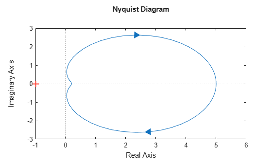
Nyquist plot of passive system

Passive systems have the following important properties for control purposes:

• The inverse of a passive system is passive.

• The parallel interconnection of passive systems is passive (see Parallel Interconnection of Passive Systems).

• The feedback interconnection of passive systems is passive (see Feedback Interconnection of Passive Systems).

When controlling a passive system with unknown or variable characteristics, it is therefore desirable to use a passive feedback law to guarantee closed-loop stability. This task can be rendered difficult given that delays and significant phase lag destroy passivity.

Directional Passivity Indices

For stability, knowing whether a system is passive or not does not tell the full story. It is often desirable to know by how much it is passive or fails to be passive. In addition, a shortage of passivity in the plant can be compensated by an excess of passivity in the controller, and vice versa. It is therefore important to measure the excess or shortage of passivity, and this is where passivity indices come into play.

There are different types of indices with different applications. One class of indices measure the excess or shortage of passivity in a particular direction of the input/output space. For example, the input passivity index is defined as the largest $$\nu$$ such that:

$${\int }_0^T{y}^T(t)u(t)dt>\nu {\int }_0^T{u}^T(t)u(t)dt,$$

for all trajectories $$y(t)=Gu(t)$$ and $$T>0$$. The system G is input strictly passive (ISP) when $$\nu >0$$, and has a shortage of passivity when $$\nu <0$$. The input passivity index is also called the input feedforward passivity (IFP) index because it corresponds to the minimum static feedforward action needed to make the system passive.

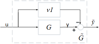
In the frequency domain, the input passivity index is characterized by:

$$\nu =\frac{1}{2}\underset{\omega }{\min }{\lambda }_{\min }(G(j\omega )+G^H(j\omega )),$$

where $${\lambda }_{\min }$$ denotes the smallest eigenvalue. In the SISO case, $$\nu$$ is the abscissa of the leftmost point on the Nyquist curve.

Similarly, the output passivity index is defined as the largest $$\rho$$ such that:

$${\int }_0^T{y}^T(t)u(t)dt>\rho {\int }_0^T{y}^T(t)y(t)dt,$$

for all trajectories $$y(t)=Gu(t)$$ and $$T>0$$. The system G is output strictly passive (OSP) when $$\rho >0$$, and has a shortage of passivity when $$\rho <0$$. The output passivity index is also called the output feedback passivity (OFP) index because it corresponds to the minimum static feedback action needed to make the system passive.

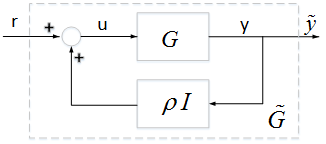
In the frequency domain, the output passivity index of a minimum-phase system $$G(s)$$ is given by:

$$\rho =\frac{1}{2}\underset{\omega }{\min }{\lambda }_{\min }(G^{-1}(j\omega )+G^{-H}(j\omega )).$$

In the SISO case, $$\rho$$ is the abscissa of the leftmost point on the Nyquist curve of $$G^{-1}(s)$$.

Combining these two notions leads to the I/O passivity index, which is the largest $$\tau$$ such that:

$${\int }_0^T{y}^T(t)u(t)dt>\tau {\int }_0^T(u^T(t)u(t)+y^T(t)y(t))dt.$$

A system with $$\tau >0$$ is very strictly passive. More generally, we can define the index in the direction $$\delta Q$$ as the largest $$\tau$$ such that:

$${\int }_0^T{y}^T(t)u(t)dt>\tau {\int }_0^T{\left(\begin{array}{c}y(t)\\ u(t)\end{array}\right)}^T\delta Q\left(\begin{array}{c}y(t)\\ u(t)\end{array}\right)dt.$$

The input, output, and I/O passivity indices all correspond to special choices of $$\delta Q$$ and are collectively referred to as directional passivity indices. You can use getPassiveIndex to compute any of these indices for linear systems in either parametric or FRD form. You can also use passiveplot to plot the input, output, or I/O passivity indices as a function of frequency. This plot provides insight into which frequency bands have weaker or stronger passivity.

There are many results quantifying how the input and output passivity indices propagate through parallel, series, or feedback interconnections. There are also results quantifying the excess of input or output passivity needed to compensate a given shortage of passivity in a feedback loop. For details, see:

• Parallel Interconnection of Passive Systems

• Series Interconnection of Passive Systems

• Feedback Interconnection of Passive Systems

Relative Passivity Index

The positive real condition for passivity:

$$G(j\omega )+G^H(j\omega )>0\forall \omega \in R,$$

is equivalent to the small gain condition:

$$||(I-G(j\omega ))(I+G(j\omega ){)}^{-1}||<1\forall \omega \in R.$$

We can therefore use the peak gain of $$(I-G)(I+G{)}^{-1}$$ as a measure of passivity. Specifically, let

$$R:={\Vert (I-G)(I+G{)}^{-1}\Vert }_{\infty }.$$

Then $$G$$ is passive if and only if $$R<1$$, and $$R>1$$ indicates a shortage of passivity. Note that $$R$$ is finite if and only if $$I+G$$ is minimum phase. We refer to $$R$$ as the relative passivity index, or R-index. In the time domain, the R-index is the smallest $$r>0$$ such that:

$${\int }_0^T||y-u|{|}^{2}dt<r^2{\int }_0^T||y+u|{|}^{2}dt,$$

for all trajectories $$y(t)=Gu(t)$$ and $$T>0$$. When $$I+G$$ is minimum phase, you can use passiveplot to plot the principal gains of $$(I-G(j\omega ))(I+G(j\omega ){)}^{-1}$$. This plot is entirely analogous to the singular value plot (see sigma), and shows how the degree of passivity changes with frequency and direction.

The following result is analogous to the Small Gain Theorem for feedback loops. It gives a simple condition on R-indices for compensating a shortage of passivity in one system by an excess of passivity in the other.

Small-R Theorem: Let $$G_1(s)$$ and $$G_2(s)$$ be two linear systems with passivity R-indices $$R_1$$ and $$R_2$$, respectively. If $$R_1{R}_2<1$$, then the negative feedback interconnection of $$G_1$$ and $$G_2$$ is stable.

References

[1] Xia, M., P. Gahinet, N. Abroug, C. Buhr, and E. Laroche. “Sector Bounds in Stability Analysis and Control Design.” International Journal of Robust and Nonlinear Control 30, no. 18 (December 2020): 7857–82. https://doi.org/10.1002/rnc.5236.