Manipulate Data for Modeling

For empirical engine modeling in the Model Browser, first load, process, and select data for modeling. This tutorial shows you how to use the Data Editor for loading data, creating variables, and creating constraints for that data.

You can load data from files (Microsoft^® Excel^® files, MATLAB^® files, text files) and from the MATLAB workspace. You can merge data in any of these forms with previously loaded data sets to produce a new data set. Test plans can use only one data set, so the merging function allows you to combine records and variables from different files in one model.

You can define new variables, apply filters to remove unwanted data, and apply operating point notes to filtered operating points. You can store and retrieve these user-defined variables and filters for any data set, and you can store plot settings. You can change and add records and apply operating point groupings, and you can match data to designs. You can also write your own data loading functions.

To get started, follow these workflow steps.

Workflow Steps	Description
View and Edit the Data	Use the Data Editor displays to investigate your data.
Create New Variables and Filters	Define your own new variables and filters to remove unwanted data.
Store and Import Variables, Filters, and Plot Preferences	Store plot preferences, user-defined variables, filters, and operating point notes.
Define Operating Point Groupings	Use the Define Operating Point Groupings dialog box to group your data.
Match Data to Experimental Designs	Use an example project to match experimental data to designs.

View and Edit the Data

Viewing Data

You can split the views to display several plots at once. Use the right-click context menus, the toolbar buttons, or the View menu to split views. You can choose 2-D plots, 3-D plots, multiple data plots, data tables, and tabs showing summary, statistics, variables, filters, operating point filters, and operating point notes. You can use operating point notes to investigate problem data and decide whether to remove some points before modeling.

Reordering and Editing Data

To change the display, right-click a 2-D plot and select Plot Properties. You can alter grid and plot settings including lines to join the data points.

Reorder X Data in the Plot Properties dialog box can be useful when record order does not produce a sensible line joining the data points. For an illustration of this:

Ensure that you are displaying a 2-D plot. You can right-click any plot and select Current Plot > 2-D Plot, or use the context menu split commands to add new views.
Right-click a 2-D plot and select Plot Properties and choose solid from the Data Linestyle drop-down menu. Click OK.
Choose afr for the y-axis.
Choose Load for the x-axis.
Select operating point 590. To use the operating point controls contained within the 2-D plot, right-click and select Separate Operating Point Selection.
Right-click and select Plot Properties and choose Reorder X Data. Click OK.
This command replots the line from left to right instead of in the order of the records, as shown.
Right-click and select Split Plot > Data Table to split the currently selected view and add a table view. You can select particular operating point numbers in the Operating Points pane on the left of the Data Editor. The Data Table will highlight data points selected in the plot with a red box. You can right-click to select Allow Editing, and then you can double-click cells to edit them.

Create New Variables and Filters

Adding New Variables

You can add new variables to the data set.

Select Tools > Variables, or click the toolbar button.
In the Variable Editor, you can define new variables in terms of existing variables. Define the new variable by writing an equation in the edit box at the top.
Define a new variable called POWER that is defined as the product of two existing variables, tq and n, by entering POWER=tq*n, as seen in the example following. You can also double-click variable names and operators to add them, which can be useful to avoid typing mistakes in variable names, which must be exact including case.
Click OK to add this variable to the current data set.
View the new variable in the Data Editor in the Variables tab at the top. You can also now see 7 + 1 variables in the summary tab.

Applying a Filter

A filter is a constraint on the data set you can use to exclude some records. You use the Filter Editor to create filters.

Choose Tools > Filters, or click the toolbar button.
In the Filter Editor, define the filter using logical operators on the existing variables.
Keep all records with speed (n) greater than 1000. Type n (or double-click the variable n), then type >1000.
Click OK to impose this filter on the current data set.
View the new filter in the Data Editor in the Filters tab at the top. Here you can see a list of your user-defined filters and how many records the new filter removes. You can also now see 141/270 records in the summary tab and a red section in the bar illustrating the records removed by the filter.

Sequence of Variables

You can change the order of user-defined variables in the Variable Editor list using the up and down arrow buttons.

Select Tools > Variables.

Example:

Define two new variables, New1 and New2. You can use the buttons to add or remove a list item to create or delete variables in this view. Click the button to 'Add item' to add a variable, and enter the definitions shown.
Notice that New2 is defined in terms of New1. New variables are added to the data in turn and hence New1 must appear in the list before New2, otherwise New2 is not well-defined.
Change the order by clicking the down arrow in the Variable Editor to produce this erroneous situation. Click OK to return to the Data Editor and in the Variables tab you can see the error message that there is a problem with the variable.
Use the arrows to order user-defined variables in legitimate sequence.

Deleting and Editing Variables and Filters

You can delete user-defined variables and filters.

Example:

To delete the added variable New1, select it in the Variables tab and press the Delete key.
You can also delete variables in the Variable Editor by clicking the Remove Item button.

Similarly, you can delete filters by selecting the unwanted filter in the Filters tab and using the Delete key.

Manually Removing Outliers

Click a point on the 2D Data Plot or Multiple Data Plots view.
The point is outlined in red on the plot, and highlighted in the data table. You can remove points you have selected as outliers by selecting Tools > Remove Data (or use the keyboard shortcut Ctrl+A). Select Tools > Restore Data (or use the keyboard shortcut Ctrl+Z) to open a dialog box where you can choose to restore any or all removed points.
You can remove individual points as outliers, or you can remove records or entire operating points with filters.
To view removed data in the table view, right-click and select Show removed data. Removed records are red. To view removed data in the 2-D and Multiple Data Plots, select Properties and select the box Show removed data.

Store and Import Variables, Filters, and Plot Preferences

You can store and import plot preferences, user-defined variables, filters, and operating point notes so they can be applied to other data sets loaded later in the session, and to other sessions.

Select Tools > Import Expressions
Click the toolbar button

The Data Editor remembers your plot type settings and when reopened displays the same types of views. You can also store your plot layouts to save the details of your Multiple Data Plots.

In the Import Variables, Filters, and Editor Layout dialog box, use the toolbar buttons to import variables, filters, and plot layouts. Import from other data sets in the current project, or from MBC project files, or from files exported from the Data Editor.

To use imported expressions in your current project, select items in the lists and click the toolbar button to apply in the data editor.

To store expressions in a file, in the Data Editor, select Tools > Export Expressions and select a file name.

Define Operating Point Groupings

The Define Operating Point Groupings dialog box records the current data object into groups. These groups are referred to as operating points.

In MATLAB, on the Apps tab, in the Automotive group, click MBC Model Fitting.
In the Model Browser home page, click Import Data.
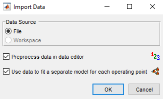
Select the checkbox Use data to fit a separate model for each operating point to automatically open the Define Operating Point Groupings dialog box.
Click OK to open a data source file.
Navigate to the matlab\toolbox\mbc\mbctraining folder. Open data file holliday.xlsx. The Data Editor opens with your data.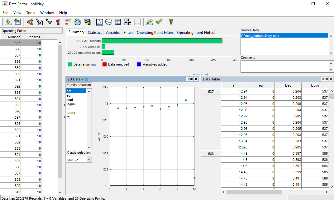
Next, the Define Operating Point Groupings dialog box will open.

The Operating Point Groupings dialog box can also be accessed from the Data Editor in either of these ways:

Using the menu Tools > Operating Point Groups
Using the toolbar button

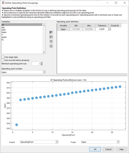
When you enter the dialog box using the holliday data, a plot is displayed as the variable logno is automatically selected for grouping operating points.

Select another variable to use in defining groups within the data.

Select n in the Variables list.
Click the button to add the variable (or double-click n).
The variable n appears in the list view on the right. You can now use this variable to define groups in the data. The maximum and minimum values of n are displayed. The Tolerance is used to define groups. When the value of n changes by more than the tolerance, a new group is defined. You change the Tolerance by typing directly in the edit box.
You can define additional groups by selecting another variable and choosing a tolerance. Data records are grouped by n or by this additional variable changing outside their tolerances.
Clear the box Group by for logno. Notice that variables can be plotted without being used to define groups.
Add load to the list by selecting it on the left and clicking .
Change the load tolerance to 0.01 and watch the operating point grouping change in the plot.
Clear the Group By check box for load. Now this variable is plotted without being used to define groups.
Blue bubbles show the operating points (groups) and the size of the blue bubble is proportional to the number of records in that operating point. You can zoom the plot by Shift-click-dragging or middle-click-dragging the mouse; zoom out again by double-clicking.
Select load in the list view (it becomes highlighted in blue) and remove it from the list by clicking the button.
Make sure that logno is selected for the Operating point number.
This changes how the operating points are displayed in the rest of the Model Browser. Operating point number can be a useful variable for identifying individual operating points in Model Browser and Data Editor views (instead of 1,2,3...) if the data was taken in numbered operating points and you want access to that information during modeling.
If you chose none from the Operating point number list, the operating points would be numbered 1,2,3, and so on, in the order in which the records appear in the data file. With logno chosen, you see operating points in the Data Editor listed as 586, 587 etc.
Every record in an operating point must share the same operating point number to identify it, so when you are using a variable to number operating points, the value of that variable is taken in the first record in each operating point.
Operating point numbers must be unique, so if any values in the chosen variable are the same, they are assigned new operating point numbers for the purposes of modeling (this does not change the underlying data, which retains the correct operating point number or other variable).
Click OK to accept the operating point groupings defined and close the dialog box.
In the Data Editor Summary tab, view the number of operating points.
The number of records shows the number of values left (after filtration) of each variable in this data set, followed by the original number of records. The color coded bars also display the number of records removed as a proportion of the total number. The values are collected into several operating points; this number is also displayed. The variables show the original number of variables plus user-defined variables.

Using Notes to Sort Data for Plotting

Right-click a view and select Current View > Multiple Plots.
Right-click the new view and select Add Plot.
The Plot Variables Setup dialog box appears.
Select spark and click to add to the X Variable box, then select tq and click to add to the Y Variable box. Click OK to create the plot.
Click in the Operating Points list to select an operating point to plot (or Shift-click, Ctrl-click, or click and drag to select multiple operating points).
Select Tools > Operating Point Notes.
In The Operating Point Note Editor, enter mean(tq)<10 in the top edit box to define the operating points to be noted, and enter Low torque in the Operating Point Note edit box. Leave the note color at the default and click OK.
Click the Operating Point Notes tab to view your note definition.
In the Operating Point Selector pane on the left, observe that all the operating points that satisfy the condition mean(tq)<10 show Low torque next to them. Click the column header to sort the operating points that meet the note condition to the top or bottom of the list.
Now create more views.
- Right-click a view and select Split View > Data Table.
- Right-click a view and select Split View > 3D Plot.
In the Operating Point Selector pane, click particular operating points with the Low torque note.
Notice that when you select an operating point here, the same operating point is plotted in the multiple data plots, the 3D data plot, and highlighted in the data table. You can use the notes in this way to easily identify problem operating points and decide whether to remove them.
For example, after examining all the Low torque noted operating points, you could decide to filter them out by applying an operating point filter.
1. Select Tools > Operating Point Filters.
2. In the Operating Point Filter Editor, enter mean(tq)>10 to keep all operating points where the mean torque is greater than 10, and click OK.
3. Click the Operating Points Filters tab and observe the new operating point filter results show it is successfully applied and the number of records removed.

Match Data to Experimental Designs

Introducing Matching Data to Designs

You can use an example project to illustrate the process of matching experimental data to designs.

Experimental data is unlikely to be identical to the desired design points. You can use the Design Match view in the Data Editor to compare the actual data collected with your experimental design points. Here you can select data for modeling. If you are interested in collecting more data, you can update your experimental design by matching data to design points to reflect the actual data collected. You can then optimally augment your design (using the Design Editor) to decide which data points it would be most useful to collect, based on the data obtained so far.

You can use an iterative process: make a design, collect some data, match that data with your design points, modify your design accordingly, then collect more data, and so on. You can use this process to optimize your data collection process to obtain the most robust models possible with the minimum amount of data.

To see the data matching functions, in the Model Browser, select File > Open Project and browse to the file Data_Matching.mat in the matlab\toolbox\mbc\mbctraining folder.
Click the Spark Sweeps node in the model tree to change to the test plan view.
Here you can see the two-stage test plan with model types and inputs set up. The global model has an associated experimental design (which you could view in the Design Editor). You are going to use the Data Editor to examine how closely the data collected so far matches to the experimental design.
Click the Edit Data button () in the toolbar.
The Data Editor appears.
You need a Design Match view to examine design and data points. Right-click a view in the Data Editor and select Current View > Design Match.
In the Design Match, you can see colored areas containing points. These are “clusters” where the matching algorithm selects closely matching design and data points.
Tolerance values (derived initially from a proportion of the ranges of the variables) are used to determine if any data points lie within tolerance of each design point. Data points that lie within tolerance of any design point are matched to that cluster. Data points that fall inside the tolerance of more than one design point form a single cluster containing all those design and data points. If no data points lie within tolerance of a design point, it remains unmatched and no cluster is plotted.
Notice the shape formed by overlapping clusters. The example shown outlined in pink is a single cluster formed where a data point lies within tolerance of two design points.
On this plot, you can see other cleared points that appear to be contained within this cluster. You track points through other factor dimensions using the axis controls to see where points are separated beyond tolerance.

Tolerances and Cluster Information

To edit tolerance values, select Tolerances in the context menu.
The Tolerance Editor appears. Here you can change the size of clusters in each dimension. Observe that the LOAD tolerance value is 100. This accounts for the elongated shape (in the LOAD dimension) of the clusters in the current plot, because this tolerance value is a high proportion of the total range of this variable.
Click the LOAD edit box and enter 20, as shown. Click OK.
Notice the change in shape of the clusters in the Design Match view.
Shift click (center-click) and drag to zoom in on an area of the plot, as shown. You can double-click to return to the full-size plot.
Click a cluster to select it. Selected points or clusters are outlined in pink. If you click and hold, you can inspect the values of global variables at the selected points (or for all data and design points if you click a cluster). You can use this information to help you decide on suitable tolerance values if you are trying to match points.
Notice that the Cluster Information list shows the details of all data and design points contained in the selected cluster. You use the check boxes here to select or exclude data or design points. Click different clusters to see various points. The list shows the values of global variables at each point, and which data and design points are within tolerance of each other. Your selections here determine which data to use for modeling, and which design points are replaced by actual data points.

Understanding Clusters

If you are not interested in collecting more data, then there is no need to make sure that the design is modified to reflect the actual data.

However, if you want your new design (called Actual Design) to accurately reflect what data has been obtained so far, for example to collect more data, then the cluster matching is important. All data points with a selected check box are added to the new Actual Design, except those in red clusters. The color of clusters indicates what proportion of selected points it contains as follows:

Green clusters have equal numbers of selected design and selected data points. The data points will replace the design points in the Actual Design.
The proportion of selected points determines the color; excluded points (with cleared check boxes) have no effect. Your check box selections can change cluster color.
Blue clusters have more data points than design points. All the data points will replace the design points in the Actual Design.
Red clusters have more design points than data points. These data points will not be added to your design as the algorithm cannot choose which design points to replace, so you must manually make selections to deal with red clusters if you want to use these data points in your design.
If you do not care about the Actual Design (for example, if you do not intend to collect more data) and you are just selecting data for modeling, then you can ignore red clusters. The data points in red clusters are selected for modeling.

Right-click the Design Match and select Select Unmatched Data. Notice that the remaining unmatched data points appear in the list. Here you can use the check boxes to select or exclude unmatched data in the same way as points within clusters.
Select a cluster, then use the drop-down menu to change the Y-Axis factor to INJ. Observe the selected cluster now plotted in the new factor dimensions of SPEED and INJ.
You can use this method to track points and clusters through the dimensions. This can give you a good idea of which tolerances to change to get points matched. Remember that points that do not form a cluster might appear to be perfectly matched when viewed in one pair of dimensions; you must view them in other dimensions to find out where they are separated beyond the tolerance value. You can use this tracking process to decide whether you want particular pairs of points to be matched, and then change the tolerances until they form part of a cluster.
Clear the Equal Data and Design check box in the Design Match view. You control what is plotted using these check boxes.
This removes the green clusters from view, as shown. These clusters are matched; you are more likely to be interested in unmatched points and clusters with uneven numbers of data and design points. Removing the green clusters allows you to focus on these points of interest. If you want your new Actual Design to accurately reflect your current data, your aim is to get as many data points matched up to design points as possible; that is, as few red clusters as possible.
Clear the check box for More Data than Design. You might also decide to ignore blue clusters, which contain more data points than design points. These design points are replaced by all data points within the cluster. An excess of data points is unlikely to be a concern.
However, blue clusters might indicate that there was a problem with the data collection at that point, and you might want to investigate why more points than expected were collected.
Select one of the remaining red clusters. Both of these have two design points within tolerance of a single data point.
Choose one of the design points to match to the data point, then clear the check box of the other design point. The cleared design point remains unchanged in the design. The selected design point is replaced by the matched data point.
Notice that the red cluster disappears. This is because your selection results in a cluster with an equal number of selected data and design points (a green cluster) and your current plot does not display green clusters.
Repeat for the other red cluster.
Now all clusters are green or blue. There are two remaining unmatched data points.
Clear the Unmatched Design check box to locate the unmatched data points. Select Unmatched Design check box again — to see design points to decide if any are close enough to the data points.
Locate and zoom in on an unmatched data point. Select the unmatched data point and a nearby design point by clicking, then use the axis drop-down menus to track the candidate pair through the dimensions. Decide if any design points are close enough to warrant changing the tolerance values to match the point with a design point.
Recall that you can right-click the Design Match and select Select Unmatched Data to display the remaining unmatched data points in the Cluster Information list. Here you can use the check boxes to select or exclude these points. If you leave them selected, they are added to the Actual Design.

These steps illustrate the process of matching data to designs, to select modeling data and to augment your design based on actual data obtained. Some trial and error is necessary to find useful tolerance values. You can select points and change plot dimensions to help you find suitable values. If you want your new Actual Design to accurately reflect your experimental data, you need to make choices to deal with red clusters. Select which design points in red clusters you want to replace with the data points. If you do not, then these data points will not be added to the new design.

When you are satisfied that you have selected all the data you want for modeling, close the Data Editor. At this point, your choices in the Design Match view are applied to the data set and a new design called Actual Design is created.

All data points with a selected check box are selected for modeling. Data points with cleared check boxes are excluded from the data set. Changes are made to the existing design to produce the new Actual Design. All selected data is added to your new design, except those in red clusters. Selected data points that have been matched to design points (in green and blue clusters) replace those design points.

All these selected data points become fixed design points (red in the Design Editor) and appear as Data in Design (pink crosses) when you reopen the Data Editor.

This means that these points will not be included in clusters when matching again. These fixed points will also not be changed in the Design Editor when you add points, though you can unlock fixed points if you want. This can be useful if you want to optimally augment a design, taking into account the data you have already obtained.