Estimate Equivalent Circuit Lithium-Ion Battery Data

R2026b

Step 1 of 2 in Characterize an Equivalent Circuit Battery

• 1
• 2

The workflow steps estimate data for an equivalent circuit lithium-ion polymer (LiPo) battery. The steps use numerical optimization techniques to determine the number of recommended RC pairs, provide initial estimates for the battery model circuit parameters, and estimate parameters to fit a model to experimental pulse discharge data. The results provide the open circuit voltage, series resistance, and RC pair parameter data.

Step 1: Load and Preprocess Data

Data Format and Requirements

The workflow supports pulse discharge sequences from 100% to 0% state-of-charge (SOC). The data requirements include:

• Time series consisting of current and voltage from an experimental pulse discharge. For each experimental data set, the temperature is constant. The sample rate should be a minimum of 1 Hz, with an ideal rate at 10 Hz.

• Voltage accuracy within ±5 mV, ideally within ±1 mV.

• Current accuracy within ±100 mA, ideally within 10 mA.

• Temperature accuracy within ±1 °C, ideally within ±1 °C.

• Change in SOC for each pulse should not be greater than 5%.

• Data collection at high or low SOC might need modification to ensure safety.

• Sufficient relaxation time after each pulse to ensure battery approaches steady-state voltage.

Load and Preprocess Data

Load and preprocess time series discharge voltage and current data for a lithium-ion polymer (LiPo) battery.

First, create a PulseSequence object.

psObj = Battery.PulseSequence;
disp(psObj);

  PulseSequence with properties:

                 Data: [0×5 double]
            ModelName: ''
             MetaData: [1×1 Battery.MetaData]
             Capacity: 1
           CapacityAh: 2.7778e-04
            NumPulses: 0
             TestType: 'none'
                 Time: [0×1 double]
              Voltage: [0×1 double]
              Current: [0×1 double]
               Charge: [0×1 double]
             ChargeAh: [0×1 double]
                  SOC: [0×1 double]
           Parameters: [1×0 Battery.Parameters]
    ParametersHistory: [1×0 Battery.Parameters]
              idxEdge: []
              idxLoad: []
             idxRelax: []
                Pulse: [0×1 Battery.Pulse]

Specify the file name and load the raw data.

FileName = 'Synthetic_LiPo_PulseDischarge.mat';
[time,voltage,current] = Battery.loadDataFromMatFile(FileName);

Add the data to the PulseSequence.

psObj.addData(time,voltage,current);

Review the pulse sequence data.

Pulse Sequence Data

psObj.plot();

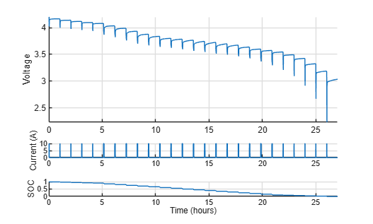
Break up the data into Battery.Pulse objects by creating the objects within the PulseSequence. This creates a parameter object with look-up tables that are the correct size.

psObj.createPulses(...
    CurrentOnThreshold=0.1,... %minimum current magnitude to identify pulse events
    NumRCBranches=3,... %how many RC pairs in the model
    RCBranchesUse2TimeConstants=false,... %do RC pairs have different time constant for discharge and rest?
    PreBufferSamples=10,... %how many samples to include before the current pulse starts
    PostBufferSamples=15); %how many samples to include after the next pulse starts

Specify the model that matches the number of RC branches and time constants.

psObj.ModelName = 'BatteryEstim3RC_PTBS';

Plot the identified pulses in the data.

Pulse Identification

psObj.plotIdentifiedPulses();

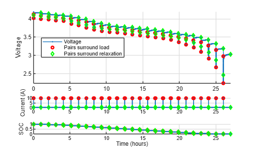
To exclude pulses, use this code.

% psObj.removePulses(indexToRemove);
% psObj.plotIdentifiedPulses();

Step 2: Determine the Number of RC Pairs

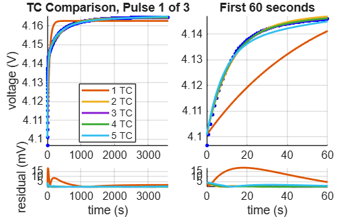
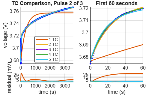
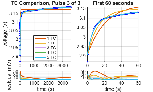
Determine the number of RC pairs. Too many pairs can over-fit the data. Too few pairs increases the fit error. If you decide to change the number of pairs, you rerun createPulses and change the NumRCBranches to the new value.

Determine the number of necessary time constants (TC) for estimation.

PulsesToTest = [1 floor(psObj.NumPulses/2), psObj.NumPulses-1];
psObj.Pulse(PulsesToTest).compareRelaxationTau();

Step 3: Estimate Parameters

Estimate the parameters. First, set parameter values. Only update parameters once. Updating the parameters changes the history.

Params = psObj.Parameters;

Params.Tx(1,:,:) = 5;
Params.Tx(2,:,:) = 50;
Params.Tx(3,:,:) = 200;

Params.TxMin(1,:,:) = 1;
Params.TxMax(1,:,:) = 50;

Params.TxMin(2,:,:) = 20;
Params.TxMax(2,:,:) = 1000;

Params.TxMin(3,:,:) = 100;
Params.TxMax(3,:,:) = 3500; %don't set this bigger than the relaxation time available

Update the parameters.

psObj.Parameters = Params;

Estimate the initial Em and R0 values. Plot the results.

psObj.estimateInitialEmR0(...
    SetEmConstraints=false,... %Update EmMin or EmMax values based on what we learn here
    EstimateEm=true,... %Keep this on to perform Em estimates
    EstimateR0=true); %Keep this on to perform R0 estimates

Parameter Tables

psObj.plotLatestParameters();

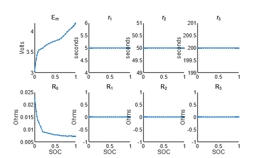
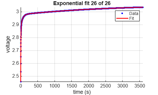
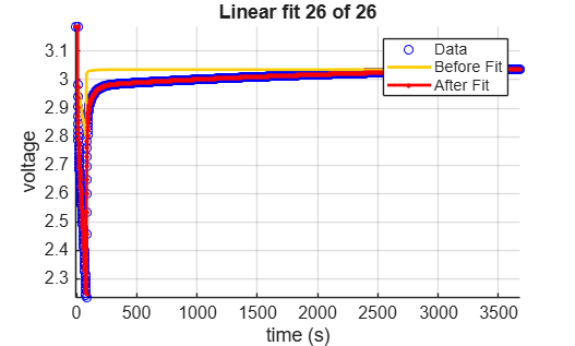
Get the initial Tx (Tau) values. This step performs curve fitting on the pulse relaxation to estimate the RC time constant at each SOC.

psObj.estimateInitialTau(...
    UpdateEndingEm=false,... %Keep this on to update Em estimates at the end of relaxations, based on the curve fit
    ShowPlots=true,... %Set this true if you want to see plots while this runs
    ReusePlotFigure=true,... %Set this true to overwrite the plots in the same figure
    UseLoadData=false,... %Set this true if you want to estimate Time constants from the load part of the pulse, instead of relaxation
    PlotDelay=0.5); %Set this to add delay so you can see the plots 

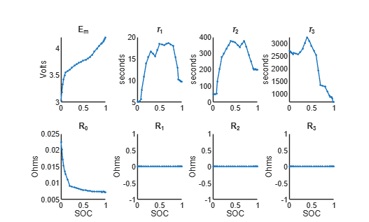
Plot the results.

Parameter Tables

psObj.plotLatestParameters();

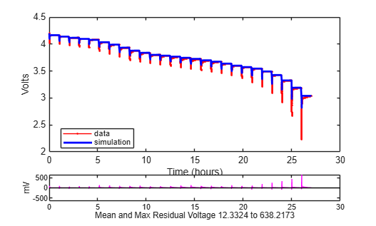
Simulation Results

psObj.plotSimulationResults(); 

Get initial Em and Rx values using a linear system approach - pulse by pulse. This step takes the data for each pulse and treats it as a linear system. It fits the Rx values for each RC branch. Optionally, you can allow it to adjust the Em and R0 values, and if these are adjusted, you also have the option whether to retain the optimized values of these or to discard them.

psObj.estimateInitialEmRx(...
    IgnoreRelaxation=false,... %Set this true if you want to ignore the relaxation periods during this step
    ShowPlots=true,...  %Set this true if you want to see plots while this runs
    ShowBeforePlots=true,... %Set this true if you want to see the 'before' value on the plots
    PlotDelay=0.5,... %Set this to add delay so you can see the plots 
    EstimateEm=true,... %Set this true to allow the optimizer to change Em further in this step
    RetainEm=true,... %Set this true keep any changes made to Em in this step
    EstimateR0=true,... %Set this true to allow the optimizer to change R0 further in this step
    RetainR0=true); %Set this true keep any changes made to R0 in this step

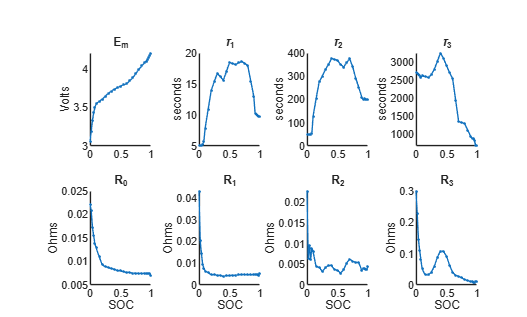
Plot the results.

Parameter Tables

psObj.plotLatestParameters();

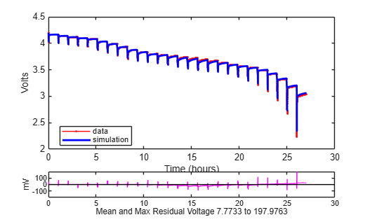
Simulation Results

psObj.plotSimulationResults(); 

Perform design optimization estimation.

SDOOptimizeOptions = sdo.OptimizeOptions(...
    OptimizedModel=psObj.ModelName,...
    Method='lsqnonlin',...
    UseParallel='always');

SDOOptimizeOptions.MethodOptions.Display = 'final';

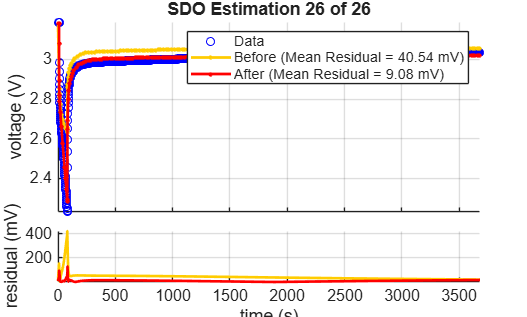
psObj.estimateParameters(...
    CarryParamToNextPulse=true,... %Set this true to use the final parameter values from the prior pulse and SOC as initial values for the next pulse and SOC
    SDOOptimizeOptions=SDOOptimizeOptions,... %Specify the SDO options object
    ShowPlots=true,... %Set this true if you want to see plots while this runs
    EstimateEm=true,... %Set this true to allow the optimizer to change Em further in this step
    RetainEm=true,... %Set this true keep any changes made to Em in this step
    EstimateR0=true,... %Set this true to allow the optimizer to change R0 further in this step
    RetainR0=true); %Set this true keep any changes made to R0 in this step

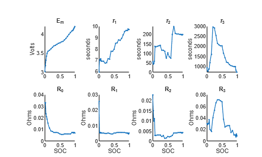
Plot the results.

Parameter Tables

psObj.plotLatestParameters();

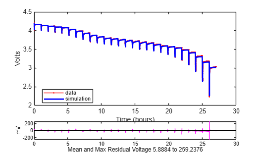
Simulation Results

psObj.plotSimulationResults();