rref
Reduced row echelon form (Gauss-Jordan elimination)
Description
Examples
Input Arguments
Output Arguments
Limitations
rank,orth, andnullare typically faster and more accurate for computing the rank and basis vectors of a matrix.mldivideis recommended to solve linear systems.
More About
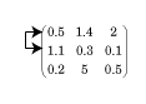
Partial pivoting is the practice of selecting the column element with largest absolute value in the pivot column, and then interchanging the rows of the matrix so that this element is in the pivot position (the leftmost nonzero element in the row).
For example, in the matrix below the algorithm starts by identifying the largest value
in the first column (the value in the (2,1) position equal to 1.1), and
then interchanges the complete first and second rows so that this value appears in the (1,1)
position.
The use of partial pivoting in Gaussian elimination reduces (but does not eliminate) roundoff errors in the calculation.
Algorithms
rref implements Gauss-Jordan elimination with partial pivoting. A
default tolerance of max(size(A))*eps*norm(A,inf) tests for negligible
column elements that are zeroed-out to reduce roundoff error.
Extended Capabilities
Version History
Introduced before R2006a