Legend Properties
Legend appearance and behavior
Legend properties control the appearance and
behavior of a Legend object. By changing property
values, you can modify certain aspects of the legend. Use dot notation to refer to a
particular object and property:
plot(rand(3))
lgd = legend('a','b','c');
c = lgd.TextColor;
lgd.TextColor = 'red';
Position and Layout
Number of columns, specified as a positive integer. If there are not enough legend items to fill the specified number of columns, then the number of columns that appear might be fewer.
Use the Orientation property to control whether the
legend items appear in order along each column or along each row.
Example: lgd.NumColumns = 3
Selection mode for the NumColumns value, specified as
one of these values:
'auto'— Automatically select the value.'manual'— Use the manually specified value. To specify the value, set theNumColumnsproperty.
Since R2023b
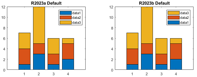
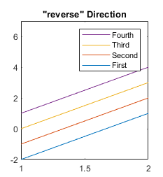
Order of legend items, specified as one of the values in this table.
For most charts, the default direction is "normal".
However, for stacked bar and area charts, the default direction is
"reverse" to match the stacking order of the
chart.
| Value | Description | Example |
|---|---|---|
| List the first item at the top and the last item at the bottom. |
|
| List the first item at the bottom and the last item at the top. |
|

Since R2023b
Selection mode for the Direction value, specified as
one of these values:
"auto"— Automatically select the value."manual"— Use the manually specified value. To specify the value, set theDirectionproperty.
Since R2024b
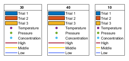
Horizontal space for legend icons, specified as a positive number in point units, where 1 point is 1/72 inch. Use this property when you want to customize the amount of space around the legend icons. Smaller values shorten the widths of certain icons, which results in less white space and a narrower legend box.
For example, here are three legends that are the same except for their
IconColumnWidth values (30,
40, and 10 respectively).
Tip
To make the region that contains the icon square, set the
IconColumnWidth property to the same value as
the FontSize
property.
lgd.IconColumnWidth = lgd.FontSize;
Since R2024b
Control how the IconColumnWidth property is set,
specified as one of these values:
"auto"— MATLAB® controls the value of theIconColumnWidthproperty depending on the icons in the legend. If the legend has only marker icons, the column shrinks to minimize the space around the icons. Otherwise, the width is30."manual"— You set the value of theIconColumnWidthproperty directly, and the width does not change.
If you set the value of the IconColumnWidth property
manually, MATLAB changes the value of the
IconColumnWidthMode property to
"manual".
Custom location and size, specified as a four-element vector of the form
[left bottom width height]. The first two values,
left and bottom, specify the
distance from the lower left corner of the figure to the lower left corner
of the legend. The last two values, width and
height, specify the legend dimensions. The
Units property determines the position units.
If you specify the Position property, then MATLAB automatically changes the Location property
to 'none'.
Example: legend({'A','B'},'Position',[0.2 0.6 0.1
0.2])
Note
Setting this property has no effect when the parent container is a
TiledChartLayout object.
Position units, specified as one of the values in this table.
Units | Description |
|---|---|
'normalized' (default) | Normalized with respect to the container, which is
usually the figure. The lower-left corner of the figure
maps to (0,0) and the upper-right
corner maps to (1,1). Resizing the
figure updates the values of the Position vector. |
'inches' | Inches. |
'centimeters' | Centimeters. |
'characters' | Based on the default system font character size.
|
'points' | Points. One point equals 1/72 inch. |
'pixels' | Pixels. On Windows® and Macintosh systems, the size of a pixel is 1/96th of an inch. This size is independent of your system resolution. On Linux® systems, the size of a pixel is determined by your system resolution. |
All units are measured from the lower-left corner of the container window.
This property affects the Position property. If you
change the units, then it is good practice to return it to its default value
after completing your computation to prevent affecting other functions that
assume Units is the default value.
If you specify the Position and
Units properties as Name,Value
pairs when creating the object, then the order of specification matters. If
you want to define the position with particular units, then you must set the
Units property before the
Position property.
Layout options, specified as a TiledChartLayoutOptions object. This property is useful when the legend is in a tiled chart layout.
To position the legend within the grid of a tiled chart layout, set
the Tile property on the TiledChartLayoutOptions
object. For example, consider a 3-by-3 tiled chart layout. The layout has a grid of tiles in
the center, and four tiles along the outer edges. In practice, the grid is invisible and the
outer tiles do not take up space until you populate them with axes or other objects.
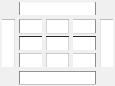
This code places the legend lgd in the third tile
of the
grid..
lgd.Layout.Tile = 3;
To place the legend in one of the surrounding tiles, specify the
Tile property as
'north',
'south',
'east', or
'west'. For example, setting the
value to 'east' places the legend in the tile
to the right of the
grid.
lgd.Layout.Tile = 'east';If the legend is not a child of a tiled chart layout (for example, if it is a child of the figure) then this property is empty and has no effect.
Labels
Automatic update of legend items to reflect the current state of the axes,
specified as "on" or "off", or as
numeric or logical 1 (true) or
0 (false). A value of
"on" is equivalent to true, and
"off" is equivalent to false.
Thus, you can use the value of this property as a logical value. The value
is stored as an on/off logical value of type matlab.lang.OnOffSwitchState.
"on"— Automatically add legend items for new graphics objects added to the axes."off"— Do not automatically add legend items.
If you delete an object from the
axes, the legend updates to reflect the change regardless of whether this
property is set to "on" or
"off". (since R2022b)
Example: legend(["A","B"],"AutoUpdate","off")
Text for legend labels, specified as a cell array of character vectors,
string array, or categorical array. To include special characters or Greek
letters in the labels, use TeX markup. For a table of options, see the
Interpreter property.
Legend title, returned as a legend text object. To add a legend title, set
the String property of the legend text object. To change
the title appearance, such as the font style or color, set legend text
properties. For a list, see Text Properties.
plot(rand(3));
lgd = legend('line 1','line 2','line 3');
lgd.Title.String = 'My Legend Title';
lgd.Title.FontSize = 12;
Alternatively, use the title function to add a
title and control the
appearance.
plot(rand(3));
lgd = legend('line 1','line 2','line 3');
title(lgd,'My Legend Title','FontSize',12)
LaTeX Markup
To use LaTeX markup, set the interpreter to "latex". For inline
mode, surround the markup with single dollar signs ($). For
display mode, surround the markup with double dollar signs
($$).
| LaTeX Mode | Example | Result |
|---|---|---|
| Inline |
"$\int_1^{20} x^2 dx$" |
|
| Display |
"$$\int_1^{20} x^2 dx$$" |
|
The displayed text uses the default LaTeX font style. The
FontName, FontWeight, and
FontAngle properties do not have an effect. To change the
font style, use LaTeX markup.
The maximum size of the text that you can use with the LaTeX interpreter is 1200 characters. For multiline text, this reduces by about 10 characters per line.
MATLAB supports most standard LaTeX math mode commands. For more information, see Supported LaTeX Commands. For examples that use TeX and LaTeX, see Greek Letters and Special Characters in Chart Text.
Font
Color and Styling
Alternatively, you can specify some common colors by name. This table lists the named color options, the equivalent RGB triplets, and the hexadecimal color codes.
| Color Name | Short Name | RGB Triplet | Hexadecimal Color Code | Appearance |
|---|---|---|---|---|
"red" | "r" | [1 0 0] | "#FF0000" |
|
"green" | "g" | [0 1 0] | "#00FF00" |
|
"blue" | "b" | [0 0 1] | "#0000FF" |
|
"cyan"
| "c" | [0 1 1] | "#00FFFF" |
|
"magenta" | "m" | [1 0 1] | "#FF00FF" |
|
"yellow" | "y" | [1 1 0] | "#FFFF00" |
|
"black" | "k" | [0 0 0] | "#000000" |
|
"white" | "w" | [1 1 1] | "#FFFFFF" |
|
"none" | Not applicable | Not applicable | Not applicable | No color |
This table lists the default color palettes for plots in the light and dark themes.
| Palette | Palette Colors |
|---|---|
Before R2025a: Most plots use these colors by default. |
|
|
|
You can get the RGB triplets and hexadecimal color codes for these palettes using the orderedcolors and rgb2hex functions. For example, get the RGB triplets for the "gem" palette and convert them to hexadecimal color codes.
RGB = orderedcolors("gem");
H = rgb2hex(RGB);
Before R2023b: Get the RGB triplets using RGB =
get(groot,"FactoryAxesColorOrder").
Before R2024a: Get the hexadecimal color codes using H =
compose("#%02X%02X%02X",round(RGB*255)).
Example: [0 0 1]
Example: 'blue'
Example: '#0000FF'
Background color, specified as an RGB triplet, a hexadecimal color code, a
color name, or a short name. The default value of [1 1 1]
corresponds to white.
For a custom color, specify an RGB triplet or a hexadecimal color code.
An RGB triplet is a three-element row vector whose elements specify the intensities of the red, green, and blue components of the color. The intensities must be in the range
[0,1], for example,[0.4 0.6 0.7].A hexadecimal color code is a string scalar or character vector that starts with a hash symbol (
#) followed by three or six hexadecimal digits, which can range from0toF. The values are not case sensitive. Therefore, the color codes"#FF8800","#ff8800","#F80", and"#f80"are equivalent.
Alternatively, you can specify some common colors by name. This table lists the named color options, the equivalent RGB triplets, and the hexadecimal color codes.
| Color Name | Short Name | RGB Triplet | Hexadecimal Color Code | Appearance |
|---|---|---|---|---|
"red" | "r" | [1 0 0] | "#FF0000" |
|
"green" | "g" | [0 1 0] | "#00FF00" |
|
"blue" | "b" | [0 0 1] | "#0000FF" |
|
"cyan"
| "c" | [0 1 1] | "#00FFFF" |
|
"magenta" | "m" | [1 0 1] | "#FF00FF" |
|
"yellow" | "y" | [1 1 0] | "#FFFF00" |
|
"black" | "k" | [0 0 0] | "#000000" |
|
"white" | "w" | [1 1 1] | "#FFFFFF" |
|
"none" | Not applicable | Not applicable | Not applicable | No color |
This table lists the default color palettes for plots in the light and dark themes.
| Palette | Palette Colors |
|---|---|
Before R2025a: Most plots use these colors by default. |
|
|
|
You can get the RGB triplets and hexadecimal color codes for these palettes using the orderedcolors and rgb2hex functions. For example, get the RGB triplets for the "gem" palette and convert them to hexadecimal color codes.
RGB = orderedcolors("gem");
H = rgb2hex(RGB);
Before R2023b: Get the RGB triplets using RGB =
get(groot,"FactoryAxesColorOrder").
Before R2024a: Get the hexadecimal color codes using H =
compose("#%02X%02X%02X",round(RGB*255)).
Example: legend({'A','B'},'Color','y')
Example: legend({'A','B'},'Color',[0.8 0.8
1])
Example: legend({'A','B'},'Color','#D9A2E9')
Box outline color, specified as an RGB triplet, a hexadecimal color code,
a color name, or a short name. The default value of [0.15 0.15
0.15] corresponds to dark gray.
For a custom color, specify an RGB triplet or a hexadecimal color code.
An RGB triplet is a three-element row vector whose elements specify the intensities of the red, green, and blue components of the color. The intensities must be in the range
[0,1], for example,[0.4 0.6 0.7].A hexadecimal color code is a string scalar or character vector that starts with a hash symbol (
#) followed by three or six hexadecimal digits, which can range from0toF. The values are not case sensitive. Therefore, the color codes"#FF8800","#ff8800","#F80", and"#f80"are equivalent.
Alternatively, you can specify some common colors by name. This table lists the named color options, the equivalent RGB triplets, and the hexadecimal color codes.
| Color Name | Short Name | RGB Triplet | Hexadecimal Color Code | Appearance |
|---|---|---|---|---|
"red" | "r" | [1 0 0] | "#FF0000" |
|
"green" | "g" | [0 1 0] | "#00FF00" |
|
"blue" | "b" | [0 0 1] | "#0000FF" |
|
"cyan"
| "c" | [0 1 1] | "#00FFFF" |
|
"magenta" | "m" | [1 0 1] | "#FF00FF" |
|
"yellow" | "y" | [1 1 0] | "#FFFF00" |
|
"black" | "k" | [0 0 0] | "#000000" |
|
"white" | "w" | [1 1 1] | "#FFFFFF" |
|
"none" | Not applicable | Not applicable | Not applicable | No color |
This table lists the default color palettes for plots in the light and dark themes.
| Palette | Palette Colors |
|---|---|
Before R2025a: Most plots use these colors by default. |
|
|
|
You can get the RGB triplets and hexadecimal color codes for these palettes using the orderedcolors and rgb2hex functions. For example, get the RGB triplets for the "gem" palette and convert them to hexadecimal color codes.
RGB = orderedcolors("gem");
H = rgb2hex(RGB);
Before R2023b: Get the RGB triplets using RGB =
get(groot,"FactoryAxesColorOrder").
Before R2024a: Get the hexadecimal color codes using H =
compose("#%02X%02X%02X",round(RGB*255)).
Example: legend({'A','B'},'EdgeColor',[0 1
0])
Since R2024a
Background transparency, specified as a scalar in the range [0, 1]. A
value of 1 is fully opaque and 0 is
completely transparent. Values between 0 and
1 are partially transparent. Here are some examples
of legends with different BackgroundAlpha
values.
| Value | Appearance |
|---|---|
|
|
|
|
|
|


Display of box outline, specified as 'on' or
'off', or as numeric or logical 1
(true) or 0
(false). A value of 'on' is
equivalent to true, and 'off' is
equivalent to false. Thus, you can use the value of this
property as a logical value. The value is stored as an on/off logical value
of type matlab.lang.OnOffSwitchState.
'on'— Display the box around the legend.'off'— Do not display the box around the legend.
Example: legend({'A','B'},'Box','off')
Interactivity
Callbacks
Callback that executes when you click legend items, specified as one of these values:
Function handle. For example,
@myCallback.Cell array containing a function handle and additional arguments. For example,
{@myCallback,arg3}.Character vector that is a valid MATLAB command or function, which is evaluated in the base workspace (not recommended).
If you specify this property using a function handle, then MATLAB passes the Legend object and
an event data structure as the first and second input arguments to the
function. This table describes the fields in the event data structure.
Event Data Structure Fields
| Field | Description |
|---|---|
Peer | Chart object associated with the clicked legend item. |
Region | Region of legend item clicked, returned as either
'icon' or
'label'. |
SelectionType | Type of click, returned as one of these values:
|
Source | Legend
object. |
EventName | Event name, 'ItemHit'. |
Note
If you set the ButtonDownFcn property, then the
ItemHitFcn property is disabled.
Example
You can create interactive legends so that when you click an item in
the legend, the associated chart updates in some way. For example, you
can toggle the visibility of the chart or change its line width. Set the
ItemHitFcn property of the legend to a callback
function that controls how the charts change. This example shows how to
toggle the visibility of a chart when you click the chart icon or label
in a legend. It creates a callback function that changes the
Visible property of the chart to either
'on' or 'off'.
Copy the following code to a new function file and save it as
hitcallback_ex1.m either in the current folder or
in a folder on the MATLAB search path. The two input arguments,
src and evnt, are the legend
object and an event data structure. MATLAB automatically passes these inputs to the callback function
when you click an item in the legend. Use the Peer
field of the event data structure to access properties of the chart
object associated with the clicked legend
item.
function hitcallback_ex1(src,evnt)

if strcmp(evnt.Peer.Visible,'on')
    evnt.Peer.Visible = 'off';
else
    evnt.Peer.Visible = 'on';
end

end
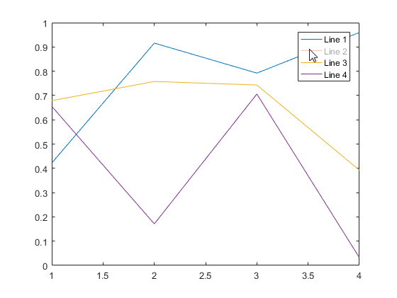
Then, plot four lines, create a legend, and assign the legend object
to a variable. Set the ItemHitFcn property of the
legend object to the callback function. Click items in the legend to
show or hide the associated chart. The legend label changes to gray when
you hide a
chart.
plot(rand(4));
l = legend('Line 1','Line 2','Line 3','Line 4');
l.ItemHitFcn = @hitcallback_ex1;
Mouse-click callback, specified as one of these values:
Function handle
Cell array in which the first element is a function handle and subsequent elements are the arguments to pass to the callback function
String scalar or character vector containing a valid MATLAB command or function, which is evaluated in the base workspace (not recommended)
The ButtonDownFcn callback executes when you click the
Legend object.
For more information on how to use function handles to define callback functions, see Create Callbacks for Graphics Objects.
Note
If the PickableParts property is set to
"none" or if the
HitTest property is set to
"off", then this callback does
not execute.
Callback Execution Control
Parent/Child
Identifiers
Version History
Introduced in R2014bThe default order of legend items for stacked (vertical) bar charts and area charts is now reversed to match the stacking order of the chart. Previously, the legend items were listed in the opposite order of stacked bars and area charts.
To preserve the order of previous releases, set the Direction
property of the legend to "normal".