Main Content

gallery

Description

[A1,A2,...,Am] = gallery(matrixname,P1,P2,...,Pn) generates a family of test matrices specified by matrixname. P1,P2,...,Pn are input parameters required by the individual matrix family. The number of input parameters P1,P2,...,Pn used in the calling syntax varies from matrix to matrix. The exact calling syntaxes for each matrix family are described in the matrixname section.

example

[A1,A2,...,Am] = gallery(matrixname,P1,P2,...,Pn,typename) additionally specifies the data type of the generated test matrices.

A = gallery(3) generates an ill-conditioned 3-by-3 matrix that is sensitive to perturbation.

example

A = gallery(5) generates a 5-by-5 matrix with an interesting eigenvalue problem that is sensitive to round-off errors.

example

Examples

collapse all

Display matrix elements of several test matrices as scaled colors.

Create a circulant matrix of size 11-by-11. A circulant matrix is a special kind of Toeplitz matrix where each row is obtained from the previous one by cyclically moving the entries one place to the right.

C = gallery('circul',11);

Display an image of the matrix elements in C. Add a colorbar to the graph to show the current colormap.

imagesc(C)
axis square
colorbar
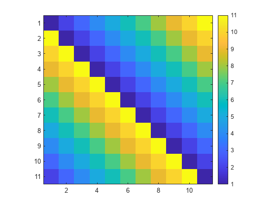
Figure contains an axes object. The axes object contains an object of type image.

Create a grcar matrix of size 11-by-11. A grcar matrix is a nonsymmetric Toeplitz matrix with -1's on the subdiagonal, 1's on the main diagonal, and 1's on the first few diagonals above the main diagonal.

G = gallery('grcar',11);

Display an image of the matrix elements in G.

imagesc(G)
axis square
colorbar
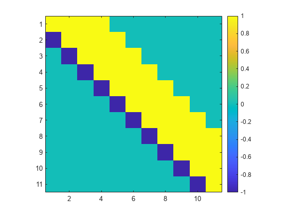
Figure contains an axes object. The axes object contains an object of type image.

Create a minij matrix of size 11-by-11. A minij matrix M is a symmetric positive definite matrix with elements M(i,j) = min(i,j).

M = gallery('minij',11);

Display an image of the matrix elements in M.

imagesc(M)
axis square
colorbar
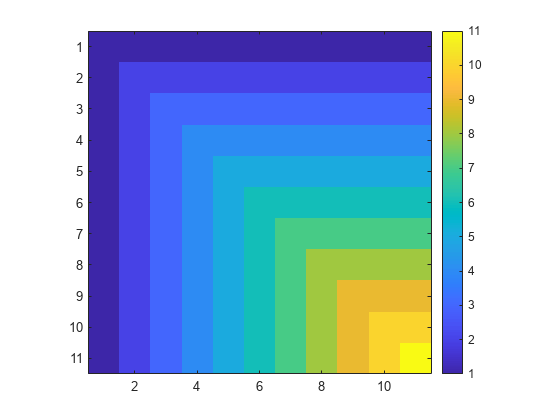
Figure contains an axes object. The axes object contains an object of type image.

An integer matrix has an inverse that is also an integer matrix if and only if its determinant is exactly 1 or –1. A square integer matrix with determinant 1 or –1 is also called a unimodular matrix. An example of such a matrix is gallery('dramadah',n), which is an n-by-n matrix of 0's and 1's with determinant 1 or –1.

Create a 6-by-6 dramadah matrix. Calculate its determinant and inverse.

A = gallery('dramadah',6)
A = 6×6

     1     1     0     1     0     0
     0     1     1     0     1     0
     0     0     1     1     0     1
     1     0     0     1     1     0
     1     1     0     0     1     1
     0     1     1     0     0     1

detA = det(A)
detA = 
-1
invA = inv(A)
invA = 6×6

    -1    -2    -3     4    -2     5
     1     1     1    -2     1    -2
    -1    -1    -2     3    -2     4
     1     1     2    -2     1    -3
     0     1     1    -1     1    -2
     0     0     1    -1     1    -1

The inverse of the matrix has only integer entries because the determinant of the original matrix is –1.

This example shows how to use Householder transformations to compute the QR decomposition of a matrix A=QR, where Q is an orthogonal matrix and R is an upper triangular matrix.

First, set the random number generator to the default value, and create a 6-by-3 rectangular matrix of random numbers from the standard normal distribution.

rng('default')
A = randn(6,3)
A = 6×3

    0.5377   -0.4336    0.7254
    1.8339    0.3426   -0.0631
   -2.2588    3.5784    0.7147
    0.8622    2.7694   -0.2050
    0.3188   -1.3499   -0.1241
   -1.3077    3.0349    1.4897

To create a Householder matrix, use the function [v,beta] = gallery('house',x). This function takes a column vector x, and returns v and β such that H=I-βvvT is a Householder matrix. The Householder transformations are used to zero out all but the first element of vector x.

Compute a Householder matrix P1 and perform the transformation A1=P1A. The matrix A1 has only zeros below the diagonal in the first column.

[v1,beta1] = gallery('house',A(:,1));
P1 = eye(6) - beta1*(v1*v1');
A1 = P1*A
A1 = 6×3

   -3.3630    2.8841    1.0421
    0.0000    1.9024    0.0858
   -0.0000    1.6571    0.5314
    0.0000    3.5028   -0.1350
    0.0000   -1.0788   -0.0983
         0    1.9227    1.3835

Next, compute a Householder matrix P2 such that A2=P2A1 has only zeros below the diagonal in the first and second columns.

[v2,beta2] = gallery('house',A1(2:end,2));
v2 = [0;v2];
P2 = eye(6) - beta2*(v2*v2');
A2 = P2*A1
A2 = 6×3

   -3.3630    2.8841    1.0421
   -0.0000   -4.8472   -0.6885
   -0.0000    0.0000    0.3413
   -0.0000    0.0000   -0.5368
    0.0000   -0.0000    0.0255
   -0.0000    0.0000    1.1630

Finally, compute a Householder matrix P3 such that A3=P3A2 has only zeros in the subdiagonal elements.

[v3,beta3] = gallery('house',A2(3:end,3));
v3 = [0;0;v3];
P3 = eye(6) - beta3*(v3*v3');
R = P3*A2
R = 6×3

   -3.3630    2.8841    1.0421
   -0.0000   -4.8472   -0.6885
    0.0000   -0.0000   -1.3258
   -0.0000    0.0000    0.0000
    0.0000   -0.0000   -0.0000
    0.0000    0.0000   -0.0000

The matrix R=P3P2P1A is an upper triangular matrix. Since the Householder matrices are involutory (the matrices are equal to their own inverses), the QR decomposition of A becomes A=QR with Q=P1P2P3.

Q = P1*P2*P3
Q = 6×6

   -0.1599   -0.0057   -0.6699    0.4983   -0.2036   -0.4857
   -0.5453   -0.3952   -0.1759   -0.6432    0.1342   -0.2895
    0.6717   -0.3386    0.1647   -0.0991    0.1551   -0.6109
   -0.2564   -0.7239    0.3290    0.5244    0.0805    0.1434
   -0.0948    0.2221   -0.0962    0.1872    0.9463   -0.0433
    0.3888   -0.3948   -0.6130   -0.1346    0.1203    0.5335

Compare this result with the computation using the qr function.

[Qa,Ra] = qr(A)
Qa = 6×6

   -0.1599   -0.0057   -0.6699    0.4983   -0.2036   -0.4857
   -0.5453   -0.3952   -0.1759   -0.6432    0.1342   -0.2895
    0.6717   -0.3386    0.1647   -0.0991    0.1551   -0.6109
   -0.2564   -0.7239    0.3290    0.5244    0.0805    0.1434
   -0.0948    0.2221   -0.0962    0.1872    0.9463   -0.0433
    0.3888   -0.3948   -0.6130   -0.1346    0.1203    0.5335

Ra = 6×3

   -3.3630    2.8841    1.0421
         0   -4.8472   -0.6885
         0         0   -1.3258
         0         0         0
         0         0         0
         0         0         0

Verify that A=QR, within machine precision.

norm(A - Q*R)
ans = 
4.7172e-15

This example plots the distribution of eigenvalues from a sample of 20,000 random circulant matrices of size 18-by-18 in the complex plane. The matrix elements are uniformly sampled from the set {–0.4,0.4}.

Create an array E of size 18-by-20,000 to store eigenvalues.

E = zeros(18,20000);

Set the random number generator to the default value. Iterate the following operations 20,000 times in a for-loop statement:

  • Create a 1-by-18 row vector x with random elements of either –0.4 or 0.4.

  • Use the vector x as an input to create a random circulant matrix A.

  • Find the eigenvalues of A and store them in E.

rng('default')
for i = 1:20000
  x = -0.4 + 0.8*randi([0 1],1,18);
  A = gallery('circul',x);
  E(:,i) = eig(A);
end

Create a scatter plot to display the eigenvalues E in the complex plane. Set the x- and y-axis limits to range from –3 to 3.

scatter(real(E(:)),imag(E(:)),'b.')
xlabel('Re(E)')
ylabel('Im(E)')
xlim([-3 3])
ylim([-3 3])
axis square
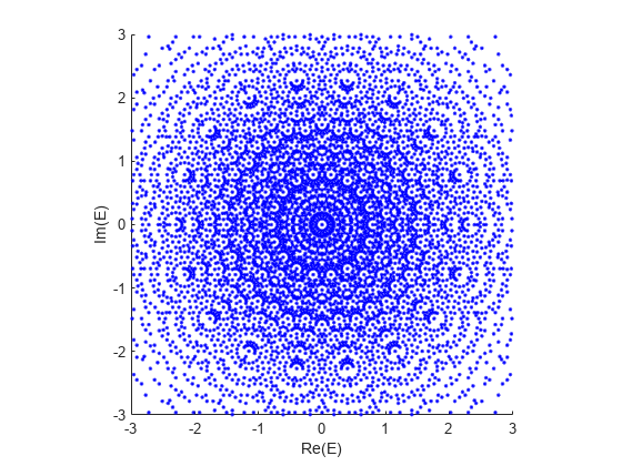
Figure contains an axes object. The axes object with xlabel Re(E), ylabel Im(E) contains an object of type scatter.

Create the test matrix gallery(3). The test matrix is ill conditioned with eigenvalues that are sensitive to perturbations.

A = gallery(3)
A = 3×3

  -149   -50  -154
   537   180   546
   -27    -9   -25

Compute the eigenvalues of A by using eig.

e = eig(A)
e = 3×1

    1.0000
    2.0000
    3.0000

Compute the eigenvalue condition numbers by using condeig.

c = condeig(A)
c = 3×1

  603.6390
  395.2366
  219.2920

The condition numbers indicate that perturbations in the matrix elements of A can result in perturbations in its eigenvalues with upper bounds that are about 200 to 600 times larger.

Next, make a small perturbation to A by adding a matrix of uniformly distributed random numbers. Set the seed of the random number generator to its default value. Add a random matrix with elements in the interval from 0 to 0.001, exclusive, to A.

rng('default')
Ap = A + 1e-3*rand(3)
Ap = 3×3

 -148.9992  -49.9991 -153.9997
  537.0009  180.0006  546.0005
  -26.9999   -8.9999  -24.9990

Compute the eigenvalues of the perturbed matrix Ap.

ep = eig(Ap)
ep = 3×1

    0.7399
    2.1437
    3.1188

Show the difference between the perturbed and the original eigenvalues.

delta = ep - e
delta = 3×1

   -0.2601
    0.1437
    0.1188

Compare the change in the eigenvalues with the upper bounds provided by the eigenvalue condition numbers. The upper bounds have roughly the same order of magnitude as the eigenvalue perturbations.

delta_upper = 1e-3*c
delta_upper = 3×1

    0.6036
    0.3952
    0.2193

Create the test matrix A = gallery(5). The test matrix has eigenvalues that are sensitive to round-off errors.

A = gallery(5)
A = 5×5

          -9          11         -21          63        -252
          70         -69         141        -421        1684
        -575         575       -1149        3451      -13801
        3891       -3891        7782      -23345       93365
        1024       -1024        2048       -6144       24572

In exact arithmetic, the matrix A has five-fold eigenvalues of λ=0 (strictly speaking, A has an eigenvalue 0 of algebraic multiplicity 5 and geometric multiplicity 1). This means that the exact characteristic polynomial of A is λ5=0. Verify that A^5 is a zero matrix.

Afifth = A^5
Afifth = 5×5

     0     0     0     0     0
     0     0     0     0     0
     0     0     0     0     0
     0     0     0     0     0
     0     0     0     0     0

Compare these results with the numerical computation of eigenvalues using eig. The eig function returns five eigenvalues of A that are small.

e = eig(A)
e = 5×1 complex

  -0.0370 + 0.0275i
  -0.0370 - 0.0275i
   0.0147 + 0.0427i
   0.0147 - 0.0427i
   0.0445 + 0.0000i

This suggests that the numerical computation of the eigenvalues of A is extremely sensitive to round-off errors due to the floating-point precision used in the computation.

Numerical computations of eigenvalues are very different from their counterparts in exact arithmetic. Instead of finding eigenvalues that are close to the exact eigenvalues of A, the eig function finds eigenvalues of a matrix that is close to A. To illustrate this, plot the exact and numerical eigenvalues of A in the complex plane.

plot(0,0,'bo',real(e),imag(e),'r*')
axis([-0.1 0.1 -0.1 0.1])
axis square
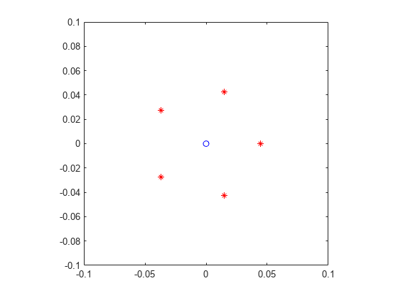
Figure contains an axes object. The axes object contains 2 objects of type line. One or more of the lines displays its values using only markers

The figure shows that the numerical eigenvalues lie on the vertices of a regular pentagon in the complex plane, centered at the origin. The radius of the pentagon is about 0.04.

Next, compute the eigenvalues of 20 matrices that are close to A. Set the random number generator to the default value, and perturb A by random numbers drawn from the standard normal distribution multiplied by eps. Plot the numerical eigenvalues of the 20 perturbed matrices.

E = zeros(20,5);
rng('default')
for i = 1:20
  E(i,:) = eig(A + eps*randn(5).*A);
end
plot(0,0,'bo',real(e),imag(e),'r*',real(E),imag(E),'k.')
axis([-0.1 0.1 -0.1 0.1])
axis square
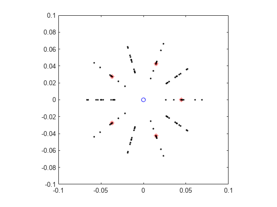
Figure contains an axes object. The axes object contains 7 objects of type line. One or more of the lines displays its values using only markers

The figure shows that the original pentagon, which represents the eigenvalues of A, can flip orientation when A is perturbed. The eigenvalues of the 20 perturbed matrices lie on the vertices of pentagons with radii in the range of 0.01 to 0.07. The computed eigenvalues of the perturbed matrices behave similarly to the computed eigenvalues of the original matrix. The inaccuracy of the computed eigenvalues is caused by the sensitivity of gallery(5).

Input Arguments

collapse all

Name of matrix family, specified as a character vector or string scalar. The argument matrixname determines the family of generated test matrices as listed below.

'binomial'

Description: Binomial matrix, which is a multiple of involutory matrix

Syntax:

  • A = gallery('binomial',n) returns an n-by-n matrix with integer entries such that A^2 = 2^(n-1)*eye(n).

Properties:

  • The matrix B = A*2^((1-n)/2) is involutory (a matrix that is its own inverse).

'cauchy'

Description: Cauchy matrix

Syntax:

  • A = gallery('cauchy',x,y) returns an n-by-n matrix with entries A(i,j) = 1/(x(i)+y(j)). Arguments x and y are vectors of length n. If you pass in scalars for x and y, they are interpreted as vectors 1:x and 1:y.

  • A = gallery('cauchy',x) returns the same as above with y = x. In other words, A(i,j) = 1/(x(i)+x(j)).

Properties:

  • Explicit formulas are known for the inverse and determinant of a Cauchy matrix.

  • The determinant det(C) is nonzero if x and y both have distinct elements.

  • C is totally positive if 0 < x(1) < ... < x(n) and 0 < y(1) < ... < y(n).

'chebspec'

Description: Chebyshev spectral differentiation matrix

Syntax:

  • A = gallery('chebspec',n,k) returns a Chebyshev spectral differentiation matrix of size n-by-n. Argument k, which can take the value 0 (default) or 1, determines the character of the output matrix.

    For k = 0 (no boundary conditions), A is nilpotent, meaning there exists a positive integer c such that A^c = 0. The matrix A has the null vector ones(n,1).

    For k = 1, A is nonsingular and well conditioned, and its eigenvalues have negative real parts.

Properties:

  • For k = 0, the matrix A is similar to a Jordan block of size n with eigenvalue zero. Two matrices A and B are called similar if there is an invertible matrix P of the same size, such that B = inv(P)*A*P.

  • For both k, the eigenvector matrix of the Chebyshev spectral differentiation matrix is ill conditioned.

'chebvand'

Description: Vandermonde-like matrix for the Chebyshev polynomials

Syntax:

  • A = gallery('chebvand',x) produces the primal Chebyshev Vandermonde matrix based on the vector of points x, which defines where the Chebyshev polynomial is calculated. Argument x is a vector of length n, and the size of A is n-by-n. The entries of A are A(i,j) = Ti – 1(x(j)), where Ti – 1 is the Chebyshev polynomial of the first kind of degree i – 1. If x is a scalar, then x equally spaced points on the interval [0,1] are used to calculate A.

  • A = gallery('chebvand',m,x) produces a rectangular version of the above with m rows, where m is a scalar.

'chow'

Description: Singular Toeplitz lower Hessenberg matrix

Syntax:

  • A = gallery('chow',n,alpha,delta) returns a Chow matrix of order n, which is an n-by-n lower Hessenberg matrix. The matrix A is defined as

    A=Hα+δI

    where the matrix elements of Hα are Hα(i,j) = α(ij + 1) for (ij + 1) ≥ 0, δ is a coefficient, and I is an n-by-n identity matrix.

  • A = gallery('chow',n) uses the default values 1 and 0 for alpha and delta, respectively.

Properties:

  • Hα has p = floor(n/2) eigenvalues that are equal to zero. The rest of the eigenvalues are equal to 4*alpha*cos(k*pi/(n+2))^2, where k = 1:(n-p).

'circul'

Description: Circulant matrix

Syntax:

  • A = gallery('circul',v) returns an n-by-n circulant matrix whose first row is the vector v of length n. A circulant matrix is a special kind of Toeplitz matrix where each row is obtained from the previous one by cyclically moving the entries one place to the right. If v is a scalar, then A = gallery('circul',1:v).

Properties:

  • The eigensystem of A is known explicitly. If t is an nth root of unity, then the inner product of v and w = [1 t t^2 ... t^(n – 1)] is an eigenvalue of A and w(n:-1:1) is an eigenvector.

See also: toeplitz

'clement'

Description: Clement tridiagonal matrix with zero diagonal entries

Syntax:

  • A = gallery('clement',n,k) returns an n-by-n tridiagonal matrix with zeros on its main diagonal. For k = 0 (default), A is nonsymmetric. For k = 1, A is symmetric.

Properties:

  • A = gallery('clement',n,1) is diagonally similar to B = gallery('clement',n,0), where there exists a diagonal matrix D of the same size such that B = inv(D)*A*D.

  • If n is odd, then A is a singular matrix.

  • The eigenvalues of A are explicitly known, which include plus and minus the numbers n-1, n-3, n-5, ..., 1 or 0.

  • The two previous properties also hold for gallery('tridiag',x,y,z), where y = zeros(n,1). If the length of the input vector y or n is odd, then gallery('tridiag',x,y,z) is singular. The eigenvalues still come in plus and minus pairs, but they are not known explicitly.

  • For odd n = 2*m+1 and k = 0, gallery('clement',n,0) has m+1 singular values that are equal to sqrt((2*m+1)^2 - (2*t+1).^2) for t = 0:m.

'compar'

Description: Comparison matrix

Syntax:

  • A = gallery('compar',B,k) returns the comparison matrix of B.

    For k = 0 (default), A(i,j) = abs(B(i,j)) if i == j and A(i,j) = -abs(B(i,j)) otherwise.

    For k = 1, A = gallery('compar',B,1) replaces each diagonal element of B with its absolute value, and replaces each off-diagonal element with the negative of the largest absolute value of off-diagonal elements within the same row.

Properties:

  • If B is triangular, then A = gallery('compar',B,1) is triangular too.

'condex'

Description: Counterexamples to matrix condition number estimators

Syntax:

  • A = gallery('condex',n,k,alpha) returns a counterexample matrix to a condition number estimator. It takes a scalar parameter alpha (default to 100) and returns a matrix of size n-by-n.

    The matrix, its natural size, and the estimator to which it applies are specified by k.

    k = 1

    4-by-4

    Counterexample to LINPACK's RCOND

    k = 2

    3-by-3

    Counterexample to LINPACK's RCOND

    k = 3

    arbitrary

    Counterexample to LINPACK's RCOND (independent of alpha)

    k = 4 (default)

    n >= 4

    Counterexample to LAPACK's RCOND (it is the inverse of this matrix that is a counter example)

    If n is not equal to the natural size of the matrix, then the matrix is padded out with an identity matrix to order n.

'cycol'

Description: Matrix whose columns repeat cyclically

Syntax:

  • A = gallery('cycol',n,k) returns an n-by-n matrix with cyclically repeating columns, where one cycle consists of the columns defined by randn(n,k). Thus, the rank of matrix A cannot exceed k, and k must be a scalar. Argument k is a scalar with default value round(n/4), and it does not need to evenly divide n.

  • A = gallery('cycol',[m n],k) returns an m-by-n matrix with cyclically repeating columns, where one cycle consists of the columns defined by randn(m,k).

'dorr'

Description: Diagonally dominant, ill-conditioned, tridiagonal matrix (sparse matrix)

Syntax:

  • A = gallery('dorr',n,theta) returns the Dorr matrix, which is an n-by-n, row diagonally dominant, tridiagonal matrix that is ill conditioned for small nonnegative values of theta. The default value of theta is 0.01.

  • [v1,v2,v3] = gallery('dorr',n,alpha) returns the vectors that define the Dorr matrix. The Dorr matrix itself is the same as gallery('tridiag',v1,v2,v3).

'dramadah'

Description: Matrix of zeros and ones

Syntax:

  • A = gallery('dramadah',n,k) returns an n-by-n matrix of 0's and 1's. n and k must both be scalars. For k = 0 and 1, mu(A) = norm(inv(A),'fro') is relatively large, although not necessarily maximal [2]. Argument k determines the character of the output matrix as listed below.

    k = 1 (default)

    A is Toeplitz and unimodular with abs(det(A)) = 1 and mu(A) > c*(1.75)^2n, where c is a constant. The inverse of A has integer entries.

    k = 2

    A is upper triangular and Toeplitz. The inverse of A has integer entries.

    k = 3

    A is Toeplitz and has maximal determinant among lower Hessenberg binary matrices (with all elements either 0 or 1). det(A) is equal to the nth Fibonacci number. The eigenvalues have an interesting distribution in the complex plane.

'fiedler'

Description: Fiedler symmetric matrix

Syntax:

  • A = gallery('fiedler',x), where x is a length n vector, returns the n-by-n symmetric matrix with elements A(i,j) = abs(x(i)-x(j)). For scalar x, A = gallery('fiedler',1:x).

Properties:

  • Matrix A has a dominant positive eigenvalue and all the other eigenvalues are negative.

  • Explicit formulas for inv(A) and det(A) are given in [3] and attributed to Fiedler. These formulas indicate that inv(A) is tridiagonal except for nonzero (1,n) and (n,1) elements.

'forsythe'

Description: Forsythe matrix or perturbed Jordan block

Syntax:

  • A = gallery('forsythe',n,alpha,lambda) returns the n-by-n matrix equal to the Jordan block with eigenvalue lambda, except that A(n,1) = alpha. The default values of scalars alpha and lambda are sqrt(eps) and 0, respectively.

Properties:

  • The characteristic polynomial of A is given by det(A-t*I) = (lambda-t)^n - alpha*(-1)^n.

'frank'

Description: Frank matrix with ill-conditioned eigenvalues

Syntax:

  • A = gallery('frank',n,k) returns the Frank matrix of size n-by-n for the default value of k = 0. The Frank matrix is an upper Hessenberg matrix with determinant 1. If k = 1, the elements are reflected about the anti-diagonal, (1,n), (2,n-1), …, (n,1).

Properties:

  • The eigenvalues of A may be obtained in terms of the zeros of the Hermite polynomials. They are positive and occur in reciprocal pairs.

  • If n is odd, then 1 is an eigenvalue.

  • The smallest half of the eigenvalues, or the smallest floor(n/2) eigenvalues, are ill conditioned.

'gcdmat'

Description: Greatest common divisor matrix

Syntax:

  • A = gallery('gcdmat',n) returns the n-by-n matrix with A(i,j) is equal to gcd(i,j).

Properties:

  • Matrix A is symmetric positive definite, and A.^r is symmetric positive semidefinite for all nonnegative r.

'gearmat'

Description: Gear matrix

Syntax:

  • A = gallery('gearmat',n,i,j) returns the n-by-n matrix with 1's on the subdiagonal and superdiagonal, sign(i) in the (1,abs(i)) position, sign(j) in the (n,n+1-abs(j)) position, and 0's everywhere else. Arguments i and j default to n and -n, respectively. They must be integers in the range of -n to n.

Properties:

  • Matrix A is singular, can have double and triple eigenvalues, and can be defective.

  • All eigenvalues are of the form 2*cos(a) and the eigenvectors are of the form [sin(w+a), sin(w+2a), …, sin(w+na)], where a and w are given in [4].

'grcar'

Description: Toeplitz matrix with sensitive eigenvalues

Syntax:

  • A = gallery('grcar',n,k) returns an n-by-n Toeplitz matrix with -1's on the subdiagonal, 1's on the main diagonal, and 1's on k diagonals above the main diagonal. k must be an integer, and the default value is k = 3. A has eigenvalues that are sensitive to perturbation.

'hanowa'

Description: Matrix whose eigenvalues lie on a vertical line in the complex plane

Syntax:

  • A = gallery('hanowa',n,alpha) returns a 2-by-2 block matrix with four n/2-by-n/2 blocks of the form:

    [alpha*eye(n/2) -diag(1:n/2)
    diag(1:n/2)     alpha*eye(n/2)]

    Argument n must be an even integer. The default value of alpha is -1. A has complex eigenvalues of the form alpha ± k*i, for 1 <= k <= n/2.

'house'

Description: Householder matrix

Syntax:

  • [v,beta] = gallery('house',x) takes x, a scalar or an n-element column vector, and returns v and beta such that H = eye(n) - beta*v*v' is a Householder matrix. A Householder matrix H satisfies the property

    H*x = -sign(x(1))*norm(x)*e1 

    where e1 is the first column of eye(n).

    Note that if x is complex, then sign(x) = exp(i*arg(x)), which is equal to x./abs(x) when x is nonzero. If x is zero, then v is zero and beta = 1.

  • [v,beta,s] = gallery('house',x,k) takes x, an n-element column vector, and returns v and beta such that H*x = s*e1. In this expression, e1 is the first column of eye(n), abs(s) = norm(x), and H = eye(n) - beta*v*v' is a Householder matrix.

    k determines the sign of s as listed below.

    k = 0 (default)

    sign(s) = -sign(x(1))

    k = 1

    sign(s) = sign(x(1))

    k = 2

    sign(s) = 1 (x must be real)

    If x is zero, or if x = alpha*e1 (alpha >= 0) and either k = 1 or k = 2, then v is zero, beta = 1, and s = x(1). In this case, H = eye(n) is the identity matrix, which is not strictly a Householder matrix.

'integerdata'

Description: Array of randomly sampled integers from uniform distribution on specified range

Syntax:

  • A = gallery('integerdata',imax,[m,n,...],k) returns an m-by-n-by-... array A whose values are a sample from the uniform distribution on the integers 1:imax. k is a random seed and must be an integer value in the interval [0,2^32-1]. Calling gallery('integerdata',...) with different values of k returns different arrays. Repeated calls to gallery('integerdata',...) with the same imax, size vector, and k always return the same array.

    In any call to gallery('integerdata',...) you can substitute individual inputs m,n,... for the size vector input [m,n,...]. For example, gallery('integerdata',7,[1,2,3,4],5) is equivalent to gallery('integerdata',7,1,2,3,4,5).

  • A = gallery('integerdata',[imin imax],[m,n,...],k) returns an m-by-n-by-... array A whose values are a sample from the uniform distribution on the integers imin:imax.

  • [A1,A2,...,Am] = gallery('integerdata',[imin imax],[m,n,...],k) returns multiple m-by-n-by-... arrays A1, A2, ..., Am containing different values.

  • [A1,A2,...,Am] = gallery('integerdata',[imin imax],[m,n,...],k,typename) produces arrays with elements of type typename. typename must be 'double' (default), 'single', 'uint8', 'uint16', 'uint32', 'int8', 'int16', or int32'.

See also: randi | rng

'invhess'

Description: Inverse of an upper Hessenberg matrix

Syntax:

  • A = gallery('invhess',x,y), where x is a length n vector and y is a length n-1 vector, returns a matrix with elements A(i,j) = x(j) if i <= j, and A(i,j) = y(i) otherwise. The lower triangle of A is based on the vector x, and the strict upper triangle is based on y. Argument y defaults to -x(1:n-1).

    For a scalar n, gallery('invhess',n) is the same as gallery('invhess',1:n).

Properties:

  • The matrix A is nonsingular if x(1) ~= 0 and x(i+1) ~= y(i) for all i.

  • The inverse of A is an upper Hessenberg matrix.

'invol'

Description: Involutory matrix (a matrix that is its own inverse)

Syntax:

  • A = gallery('invol',n) returns an n-by-n involutory matrix, where A*A = eye(n) and A is ill conditioned. It is a diagonally scaled version of hilb(n).

Properties:

  • The matrices B = (eye(n)-A)/2 and B = (eye(n)+A)/2 are idempotent, where B*B = B.

See also: hilb

'ipjfact'

Description: Hankel matrix with factorial elements

Syntax:

  • [A,beta] = gallery('ipjfact',n,k) returns an n-by-n Hankel matrix A and its determinant beta, which is known explicitly. The inverse of A is also known explicitly.

    If k = 0 (default), then the elements of A are A(i,j) = factorial(i+j). If k = 1, then the elements of A are A(i,j) = 1/factorial(i+j).

See also: hankel | toeplitz

'jordbloc'

Description: Jordan block matrix

Syntax:

  • A = gallery('jordbloc',n,lambda) returns the n-by-n Jordan block with eigenvalue lambda. The default value for lambda is 1.

'kahan'

Description: Upper trapezoidal Kahan matrix

Syntax:

  • A = gallery('kahan',n,theta,pert) returns an upper trapezoidal matrix that has interesting properties regarding estimation of condition and rank. For example, the Kahan matrix illustrates that using a column-permuted QR decomposition can fail to give a good rank estimation of a matrix.

    If n is a two-element vector, then A is n(1)-by-n(2); otherwise, A is n-by-n. The useful range of theta is 0 < theta < pi, with a default value of 1.2.

    To ensure that the QR factorization with column pivoting does not interchange columns in the presence of rounding errors, the main diagonal is perturbed by pert*eps*diag([n:-1:1]). The default value of pert is 1e3, which ensures no interchanges for gallery('kahan',n) up to at least n = 100 in IEEE® arithmetic (for default value of theta = 1.2).

'kms'

Description: Kac-Murdock-Szegö Toeplitz matrix

Syntax:

  • A = gallery('kms',n,rho) returns the n-by-n Kac-Murdock-Szegö Toeplitz matrix such that A(i,j) = rho^(abs(i-j)) for real rho. For complex rho, the same formula holds except that elements below the diagonal are conjugated. rho defaults to 0.5.

Properties:

  • There exists an LDL factorization of A with L = inv(gallery('triw',n,-rho,1))', and D = (1-abs(rho)^2)*eye(n), except the first element of D is D(1,1) = 1.

  • A is positive definite if and only if 0 < abs(rho) < 1.

  • The inverse inv(A) is tridiagonal.

'krylov'

Description: Krylov matrix

Syntax:

  • A = gallery('krylov',B,x,k) returns the Krylov matrix, where B is an n-by-n matrix, x is a vector with length n, and k must be an integer. The Krylov matrix is equal to

    [x, B*x, B^2*x, ..., B^(k-1)*x]

    for a column vector x. If you do not specify the arguments x and k, they take the default values of x = ones(n,1) and k = n.

  • A = gallery('krylov',n) for a scalar n is the same as gallery('krylov',B) with B = randn(n).

'lauchli'

Description: Lauchli rectangular matrix

Syntax:

  • A = gallery('lauchli',n,mu) returns the (n+1)-by-n matrix of the form [ones(1,n); mu*eye(n)]. Argument mu defaults to sqrt(eps).

Properties:

  • The Lauchli matrix is a well-known example in least squares and other problems that shows the dangers of forming A'*A when solving the equation ATAx^=ATb. The matrix A'*A is in general more sensitive to rounding errors than the initial matrix A.

'lehmer'

Description: Lehmer symmetric positive definite matrix

Syntax:

  • A = gallery('lehmer',n) returns the symmetric positive definite n-by-n matrix such that A(i,j) = i/j for j >= i and A(i,j) = j/i otherwise.

Properties:

  • A is totally nonnegative.

  • The inverse inv(A) is tridiagonal and explicitly known.

  • The order n satisfies n <= cond(A) <= 4*n*n.

'leslie'

Description: Matrix of birth numbers and survival rates from the Leslie population model

Syntax:

  • A = gallery('leslie',x,y) is the n-by-n matrix from the Leslie population model with average birth numbers x(1:n) and survival rates y(1:n-1). The matrix elements are mostly zero, apart from the first row that contains x(i) and the first subdiagonal that contains y(i). For a valid model, the elements of x are nonnegative, and the elements of y are positive and bounded by 1, where 0 < y(i) <= 1.

  • A = gallery('leslie',n) generates the Leslie matrix with x = ones(n,1) and y = ones(n-1,1).

'lesp'

Description: Tridiagonal matrix with real, sensitive eigenvalues

Syntax:

  • A = gallery('lesp',n) returns an n-by-n matrix whose eigenvalues are real and smoothly distributed in the interval [-2*n-3.5,-4.5].

Properties:

  • The sensitivities of the eigenvalues increase exponentially as the eigenvalues grow more negative.

  • The matrix is similar to the symmetric tridiagonal matrix B with the same diagonal entries and with off-diagonal entries 1 via a similarity transformation A = inv(D)*B*D, where D = diag(factorial(1:n)).

'lotkin'

Description: Lotkin matrix

Syntax:

  • A = gallery('lotkin',n) returns the Hilbert matrix with its first row altered to all 1's.

Properties:

  • The Lotkin matrix A is nonsymmetric, ill conditioned, and has many negative eigenvalues of small magnitude.

  • Its inverse has integer entries and is known explicitly [5].

'minij'

Description: Symmetric positive definite matrix

Syntax:

  • A = gallery('minij',n) returns the n-by-n symmetric positive definite matrix with entries A(i,j) = min(i,j).

Properties:

  • A has eigenvalues of 0.25*sec(r*pi/(2*n+1)).^2, where r = 1:n.

  • The inverse inv(A) is tridiagonal and equal to -1 times the second difference matrix, except its (n,n) element is 1.

  • The matrix 2*A-ones(size(A)) has tridiagonal inverse and eigenvalues of 0.5*sec((2*r-1)*pi/(4*n)).^2, where r = 1:n.

'moler'

Description: Moler symmetric positive definite matrix

Syntax:

  • A = gallery('moler',n,alpha) returns the symmetric positive definite n-by-n matrix U'*U, where U = gallery('triw',n,alpha). For the default value of alpha = -1, A(i,j) = min(i,j)-2, and A(i,i) = i.

Properties:

  • For alpha = -1, one of the eigenvalues of A is small, which differs by many orders of magnitude compared to the rest of the eigenvalues.

'neumann'

Description: Singular matrix from the discrete Neumann problem (sparse matrix)

Syntax:

  • A = gallery('neumann',n) returns the sparse n-by-n singular, row diagonally dominant matrix resulting from discretizing the Neumann problem with the usual five-point operator on a regular mesh. Argument n must be a perfect square integer. A is sparse and has a one-dimensional null space with null vector ones(n,1).

  • A = gallery('neumann',[m n]) returns an identical matrix, but with size m*n-by-m*n. Arguments m and n must be positive integers, where m must be larger than 1.

'normaldata'

Description: Array of randomly sampled numbers from standard normal (Gaussian) distribution

Syntax:

  • A = gallery('normaldata',[m,n,...],k) returns an m-by-n-by-... array A. The elements of A are a random sample of numbers from the standard normal distribution. k is a random seed and must be an integer value in the interval [0, 2^32-1]. Calling gallery('normaldata',...) with different values of k returns different arrays. Repeated calls to gallery('normaldata',...) with the same size vector [m,n,...] and the same value of k always return the same array.

    In any call to gallery('normaldata',...) you can substitute individual inputs m,n,... for the size vector input [m,n,...]. For example, gallery('normaldata',[1,2,3,4],5) is equivalent to gallery('normaldata',1,2,3,4,5).

  • [A1,A2,...,Am] = gallery('normaldata',[m,n,...],k) returns multiple m-by-n-by-... arrays A1, A2, ..., Am containing different values.

  • [A1,A2,...,Am] = gallery('normaldata',[m,n,...],k,typename) produces arrays with elements of type typename. typename must be either 'double'(default) or 'single'.

See also: randn | rng

'orthog'

Description: Orthogonal and nearly orthogonal matrices

Syntax:

  • A = gallery('orthog',n,k) returns the kth type of matrix of order n, where k > 0 returns exactly orthogonal matrices, and k < 0 returns different diagonal scalings of orthogonal matrices.

    k = 1 (default)

    A(i,j) = sqrt(2/(n+1)) * sin(i*j*pi/(n+1))

    Matrix of eigenvectors of the second difference matrix gallery('tridiag',n). A is symmetric and orthogonal.

    k = 2

    A(i,j) = 2/(sqrt(2*n+1)) * sin(2*i*j*pi/(2*n+1))

    Symmetric and orthogonal matrix.

    k = 3

    A(r,s) = exp(2*pi*i*(r-1)*(s-1)/n) / sqrt(n)

    Complex matrix that is unitary. A^4 is an identity matrix. This is exactly the same matrix as fft(eye(n))/sqrt(n).

    k = 4

    Standard Helmert matrix: a permutation of a lower Hessenberg matrix, whose first row is ones(1,n)/sqrt(n).

    k = 5

    A(i,j) = sin(2*pi*(i-1)*(j-1)/n)/sqrt(n) + cos(2*pi*(i-1)*(j-1)/n)/sqrt(n)

    Symmetric matrix arising in the Hartley transform.

    k = 6

    A(i,j) = sqrt(2/n) * cos((i-1/2)*(j-1/2)*pi/n)

    Symmetric matrix arising as a discrete cosine transform.

    k = -1

    A(i,j) = cos((i-1)*(j-1)*pi/(n-1))

    Chebyshev Vandermonde-like matrix, based on the extrema of Chebyshev polynomial of the first kind T(n-1). This matrix is symmetric. Each even column (row) vector of the matrix is orthogonal to each odd column (row) vector, that is A(i,:)*A(j,:)' = 0 for any even i and odd j.

    k = -2

    A(i,j) = cos((i-1)*(j-1/2)*pi/n)

    Chebyshev Vandermonde-like matrix, based on the zeros of T(n). This matrix has row vectors that are orthogonal to each other, that is A(i,:)*A(j,:)' = 0 for i not equal to j. The matrix A*A' is not the identity matrix, but it is a diagonal matrix.

'parter'

Description: Parter matrix

Syntax:

  • A = gallery('parter',n) returns the matrix A such that A(i,j) = 1/(i-j+0.5).

Properties:

  • A is a Cauchy and Toeplitz matrix.

  • Most of the singular values of A are very close to pi.

'pei'

Description: Pei matrix

Syntax:

  • A = gallery('pei',n,alpha), where alpha is a scalar, returns the symmetric matrix alpha*eye(n) + ones(n). The default value for alpha is 1. The matrix is singular for alpha equal to either 0 or -n.

'poisson'

Description: Block tridiagonal matrix from Poisson's equation (sparse matrix)

Syntax:

  • A = gallery('poisson',n) returns the sparse block tridiagonal matrix of order n^2 resulting from discretizing Poisson's equation with the 5-point operator on an n-by-n mesh.

'prolate'

Description: Prolate matrix

Syntax:

  • A = gallery('prolate',n,alpha) returns the n-by-n prolate matrix with parameter alpha. It is a symmetric, ill-conditioned Toeplitz matrix. If 0 < alpha < 0.5, then A is positive definite.

Properties:

  • The eigenvalues of A are distinct, lie in the interval (0,1), and tend to cluster around 0 and 1.

  • The default value of w is 0.25.

'randcolu'

Description: Random matrix with normalized columns and specified singular values

Syntax:

  • A = gallery('randcolu',n) generates a random n-by-n matrix with normalized columns of unit 2-norm and random singular values from a uniform distribution.

    A'*A is a correlation matrix of the similar form of that produced by gallery('randcorr',n). The eigenvalues of the latter are uniformly distributed, while for the former, the square roots of the eigenvalues are uniformly distributed.

  • A = gallery('randcolu',x), where x is a vector of length n (n > 1), produces a random n-by-n matrix with singular values given by the vector x. The vector x must have nonnegative elements whose sum of squares is n. This matrix also has normalized columns of unit 2-norm.

  • A = gallery('randcolu',__,m), where m >= n, produces an m-by-n matrix.

  • A = gallery('randcolu',__,m,k) provides additional options based on k.

    k = 0 (default)

    diag(x) is initially subjected to a random two-sided orthogonal transformation, and then a sequence of Givens rotations is applied.

    k = 1

    The initial transformation is omitted. This is faster when generating the test matrix, but the resulting matrix typically has many zero entries.

'randcorr'

Description: Random correlation matrix with specified eigenvalues

Syntax:

  • A = gallery('randcorr',n) is a random n-by-n correlation matrix with random eigenvalues from a uniform distribution. A correlation matrix is a symmetric positive semi-definite matrix with 1's on the diagonal.

  • A = gallery('randcorr',x) produces a random correlation matrix with eigenvalues given by the vector x, where length(x) > 1. The vector x must have nonnegative elements whose sum is length(x).

  • A = gallery('randcorr',x,k) provides additional options based on k.

    k = 0 (default)

    The diagonal matrix of eigenvalues is initially subjected to a random orthogonal similarity transformation, and then a sequence of Givens rotations is applied [6].

    k = 1

    The initial transformation is omitted. This is faster when generating the test matrix, but the resulting matrix typically has many zero entries.

See also: corrcoef

'randhess'

Description: Random, orthogonal upper Hessenberg matrix

Syntax:

  • A = gallery('randhess',n) returns an n-by-n real, random, orthogonal upper Hessenberg matrix.

  • A = gallery('randhess',x) constructs A nonrandomly using the elements of x as parameters. x must be a real vector with length n, where n > 1.

    In both cases, matrix A is constructed from a product of n-1 Givens rotations.

'randjorth'

Description: Random J-orthogonal matrix

Syntax:

  • A = gallery('randjorth',n) produces a random n-by-n J-orthogonal matrix A that satisfies the relation A'*J*A = J (such matrices are also known as hyperbolic). Here, J = blkdiag(eye(ceil(n/2)),-eye(floor(n/2))), and cond(A) = sqrt(1/eps).

  • A = gallery('randjorth',n,m), for positive integers n and m, produces a random (n+m)-by-(n+m) J-orthogonal matrix A. Here, J = blkdiag(eye(n),-eye(m)), and cond(A) = sqrt(1/eps).

  • A = gallery('randjorth',n,m,alpha,symm,method)

    uses the following optional input arguments:

    • alpha — Specify cond(A) = alpha, where alpha must be equal to or larger than 1.

    • symm — Choose to enforce symmetry or not. A is nonsymmetric if the scalar symm is 0. A is symmetric if the scalar symm is 1 or nonzero.

    • method — Choose to call qr to perform the underlying orthogonal transformations or not. qr is not called if the scalar method is 0. qr is called if the scalar method is 1 or nonzero. A call to qr is much faster than the default method to create the J-orthogonal matrix for large dimensions.

'rando'

Description: Random matrix composed of elements –1, 0 or 1

Syntax:

  • A = gallery('rando',n,k) returns a random n-by-n matrix. The input argument k determines the matrix elements from one of the following discrete distributions.

    k = 1 (default)

    A(i,j) = 0 or 1 with equal probability.

    k = 2

    A(i,j) = -1 or 1 with equal probability.

    k = 3

    A(i,j) = -1, 0, or 1 with equal probability.

  • A = gallery('rando',[n m],k) returns a random n-by-m matrix.

'randsvd'

Description: Random matrix with preassigned singular values

Syntax:

  • A = gallery('randsvd',n,kappa,mode,kl,ku) returns a banded (multidiagonal) random matrix of order n with condition number cond(A) = abs(kappa), which must be larger or equal than 1. If n is a two-element vector, A has the size of n(1)-by-n(2).

    The default value of kappa is sqrt(1/eps). The distribution mode mode determines the singular values of the matrix.

    Arguments kl and ku specify the number of lower and upper off-diagonals in A, respectively. If they are omitted, a full matrix is produced with kl = n-1 and ku = kl. If only kl is present, ku defaults to kl.

    Available values of mode are listed below.

    mode = 1

    One large singular value that is equal to 1 (and the rest of the singular values are equal to 1/abs(kappa)).

    mode = 2

    One small singular value that is equal to 1/abs(kappa) (and the rest of the singular values are equal to 1).

    mode = 3 (default)

    Geometrically distributed singular values.

    mode = 4

    Arithmetically distributed singular values.

    mode = 5

    Random singular values with uniformly distributed logarithm.

    mode < 0

    If mode is -1, -2, -3, -4, or -5, then randsvd treats mode as abs(mode). However, in the original matrix of singular values, the order of the diagonal entries is reversed from small to large instead of from large to small.

    In the special case of kappa <= 1, A is a symmetric, positive definite matrix with cond(A) = -kappa and eigenvalues distributed according to mode. In this case, the arguments kl and ku are ignored.

  • A = gallery('randsvd',n,kappa,mode,kl,ku,method) specifies how the computations to generate the test matrix are carried out. method = 0 is the default, while method = 1 uses an alternative method to call qr that is much faster for large dimensions, even though it uses more floating-point operations per second.

'redheff'

Description: Redheffer matrix of ones and zeros

Syntax:

  • A = gallery('redheff',n) returns an n-by-n matrix of 0's and 1's defined by A(i,j) = 1, if j = 1 or if i divides j, and A(i,j) = 0 otherwise.

Properties:

  • A has n-floor(log2(n))-1 eigenvalues that are equal to 1.

  • A has a real eigenvalue (and its spectral radius) that is approximately sqrt(n).

  • A has a negative eigenvalue that is approximately -sqrt(n).

  • The remaining floor(log2(n))-1 eigenvalues have relatively small moduli, which lie inside the circle log2εn, for ε > 0 and large enough n.

  • The Riemann hypothesis is true if and only if |det(A)|=O(n1/2+ε) for every ε > 0.

  • Barrett and Jarvis conjecture that floor(log2(n)) of the small eigenvalues lie inside the unit circle abs(z) = 1. A proof of this conjecture, together with a proof that some eigenvalues tend to zero as n tends to infinity, would yield a new proof of the prime-number theorem [7].

'riemann'

Description: Matrix associated with the Riemann hypothesis

Syntax:

  • A = gallery('riemann',n) returns an n-by-n matrix for which the Riemann hypothesis is true if and only if

    det(A)=O(n!n1/2+ε)

    for every ε > 0 [8].

    The Riemann matrix is defined by A = B(2:n+1,2:n+1), where B(i,j) = i-1 if i divides j, and B(i,j) = -1 otherwise.

Properties:

  • Each eigenvalue e(i) satisfies abs(e(i)) <= m-1/m, where m = n+1.

  • The eigenvalues also satisfies i <= e(i) < i+1, with at most m-sqrt(m) exceptions.

  • All integers in the interval (m/3,m/2] are eigenvalues.

'ris'

Description: Ris matrix

Syntax:

  • A = gallery('ris',n) returns a symmetric n-by-n Hankel matrix with elements A(i,j) = 0.5/(n-i-j+1.5). The eigenvalues of A cluster around π/2 and –π/2.

'sampling'

Description: Nonsymmetric matrix with ill-conditioned integer eigenvalues

Syntax:

  • A = gallery('sampling',x), where x is a vector of length n, returns an n-by-n nonsymmetric matrix. The elements of the matrix are A(i,j) = x(i)/(x(i)-x(j)) for i ~= j and A(j,j) equals to the sum of the off-diagonal elements in column j. If x is a scalar, then A = gallery('sampling',1:x).

Properties:

  • A has integer eigenvalues 0:n-1 that are ill conditioned.

  • For the eigenvalues 0 and n-1, the corresponding eigenvectors are x and ones(n,1), respectively.

  • A has the property that A(i,j) + A(j,i) = 1 for i ~= j.

  • Explicit formulas are available for the left eigenvectors of A.

  • A special case of this matrix has appeared in sampling theory where its right eigenvectors, if properly normalized, give the inclusion probabilities of the conditional Poisson sampling design [9].

'smoke'

Description: Complex matrix with a "smoke ring" pseudospectrum

Syntax:

  • A = gallery('smoke',n) returns an n-by-n matrix with 1's on the superdiagonal and 1 in the (n,1) position. The diagonal consists of the set of all nth roots of unity.

  • A = gallery('smoke',n,1) returns the same as above except that the element A(n,1) is zero.

Properties:

  • The eigenvalues of gallery('smoke',n,1) are the nth roots of unity.

  • The eigenvalues of gallery('smoke',n) are the nth roots of unity times 2^(1/n).

  • The pseudospectrum of a matrix A can be calculated by finding the minimum singular value of the matrix zI-A in the complex plane. Here, z represents points in the complex plane, and I is an identity matrix. The pseudospectra of gallery('smoke',n) and gallery('smoke',n,1) have "smoke ring" patterns near their eigenvalues.

'toeppd'

Description: Symmetric positive definite Toeplitz matrix

Syntax:

  • A = gallery('toeppd',n,m,x,theta) returns an n-by-n symmetric Toeplitz matrix composed of the sum of m Toeplitz matrices (with rank 1 or 2). x and theta are vectors of length m. The matrix A is positive definite if all elements of x are positive. Specifically, A is generated by

    A = x(1)*T1 + ... + x(k)*Tk + ... + x(m)*Tm

    where Tk is an n-by-n matrix that depends on theta(k). The elements of Tk are Tk(i,j) = cos(2*pi*theta(k)*(i-j)).

    By default, m = n, x = rand(m,1), and theta = rand(m,1).

'toeppen'

Description: Pentadiagonal Toeplitz matrix (sparse matrix)

Syntax:

  • A = gallery('toeppen',n,a,b,c,d,e) returns the n-by-n sparse pentadiagonal Toeplitz matrix with elements: a on the second diagonal below the main diagonal, b on the subdiagonal, c on the main diagonal, d on the superdiagonal, and e on the second diagonal above the main diagonal, where a, b, c, d, and e are scalars.

    By default, (a,b,c,d,e) = (1,-10,0,10,1), yielding a matrix that was originally introduced by Rutishauser [10]. This matrix has eigenvalues lying approximately on the curve 2*cos(2*t) + 20*i*sin(t) in the complex plane.

'tridiag'

Description: Tridiagonal matrix (sparse matrix)

Syntax:

  • A = gallery('tridiag',n) returns the sparse tridiagonal matrix of size n-by-n with subdiagonal elements -1, diagonal elements 2, and superdiagonal elements -1. This matrix has eigenvalues 2 + 2*cos(k*pi/(n+1)), where k = 1:n.

    The generated matrix is a symmetric positive definite M-matrix with real nonnegative eigenvalues. This matrix is also the negative of the second difference matrix.

  • A = gallery('tridiag',c,d,e) returns the tridiagonal matrix with subdiagonal c, diagonal d, and superdiagonal e defined by the vectors c, d, and e. The length of vectors c and e must be length(d)-1.

  • A = gallery('tridiag',n,c,d,e), where c, d, and e are all scalars, yields the Toeplitz tridiagonal matrix of size n-by-n with subdiagonal elements c, diagonal elements d, and superdiagonal elements e. This matrix has eigenvalues d + 2*sqrt(c*e)*cos(k*pi/(n+1)), where k = 1:n.

'triw'

Description: Upper triangular matrix discussed by Wilkinson and others

Syntax:

  • A = gallery('triw',n,alpha,k) returns the upper triangular matrix with 1's on the diagonal and alpha's on the first k >= 0 superdiagonals. By default, alpha = -1, and k = n-1.

    The order n can be a 2-element vector, in which case the matrix is n(1)-by-n(2) and upper trapezoidal.

Properties:

  • For alpha = 2, the condition number of the matrix satisfies:

    cond(gallery('triw',n,2)) = cot(pi/(4*n))^2,
  • For large abs(alpha), cond(gallery('triw',n,alpha)) is approximately abs(alpha)^n*sin(pi/(4*n-2)).

  • The matrix A = gallery('triw',n) becomes singular when you add -2^(2-n) to its (n,1) element. The matrix also becomes singular when you add -2^(1-n) to its elements in the first column.

'uniformdata'

Description: Array of randomly sampled numbers from standard uniform distribution

Syntax:

  • A = gallery('uniformdata',[m,n,...],k) returns an m-by-n-by-... array A. The elements of A are a random sample of numbers from the standard uniform distribution. k is a random seed and must be an integer value in the interval [0, 2^32-1]. Calling gallery('uniformdata',...) with different values of k returns different arrays. Repeated calls to gallery('uniformdata',...) with the same size vector [m,n,...] and the same value of k always return the same array.

    In any call to gallery('uniformdata',...) you can substitute individual inputs m,n,... for the size vector input [m,n,...]. For example, gallery('uniformdata',[1,2,3,4],5) is equivalent to gallery('uniformdata',1,2,3,4,5).

  • [A1,A2,...,Am] = gallery('uniformdata',[m,n,...],k) returns multiple m-by-n-by-... arrays A1, A2, ..., Am containing different values.

  • [A1,A2,...,Am] = gallery('uniformdata',[m,n,...],k,typename) produces arrays with elements of type typename. typename must be either 'double' (default) or 'single'.

See also: rand | rng

'wathen'

Description: Wathen matrix (sparse matrix)

Syntax:

  • A = gallery('wathen',nx,ny) returns a sparse, random, n-by-n finite element matrix where n = 3*nx*ny + 2*nx + 2*ny + 1.

    Matrix A is precisely the “consistent mass matrix” for a regular nx-by-ny grid of 8-node (serendipity) elements in two dimensions. A is symmetric, positive definite for any (positive) values of the “density” rho(nx,ny), which is chosen randomly.

  • B = gallery('wathen',nx,ny,1) returns a diagonally scaled matrix based on the previous syntax, where B = diag(diag(A))\A. The eigenvalues of this matrix satisfy

    0.25 <= eig(B) <= 4.5

    for any positive integers nx and ny and any densities rho(nx,ny).

'wilk'

Description: Various matrices devised or discussed by Wilkinson

Syntax:

  • [U,b] = gallery('wilk',3) returns an upper triangular system U*x = b illustrating an inaccurate solution.

  • [L,b] = gallery('wilk',4) returns a lower triangular system L*x = b, which is ill conditioned.

  • A = gallery('wilk',5) returns a symmetric positive definite matrix A = B(1:5,2:6)*1.8144, where B = hilb(6).

  • A = gallery('wilk',21) returns W21+, a tridiagonal matrix with pairs of nearly equal eigenvalues. For more details, see [11].

Input parameters, specified as scalars, vectors, or matrices. The parameters P1,P2,...,Pn used in the calling syntax depend on the matrix family as discussed in the table in matrixname.

Data type of generated test matrices, specified as a character vector or string scalar.

  • If typename is not specified, then the data type of the output matrices is determined from those arguments among P1,P2,...,Pn that do not specify matrix dimensions or select an option to determine the character of the output matrices. If any of these arguments is of data type single, then the output data type is single. Otherwise, the output data type is double.

  • typename must be either 'double' or 'single' for all test matrices, unless matrixname is 'integerdata'. If matrixname is 'integerdata', then typename can be 'double', 'single', 'int8', 'int16', 'int32', 'uint8', 'uint16', or 'uint32'.

Output Arguments

collapse all

Output coefficients, vectors, matrices, or multidimensional arrays. The outputs A1,A2,...,Am that are generated by the calling syntax depend on the matrix family as discussed in the table in matrixname. In most cases, the gallery function only returns one matrix as the output argument.

Output matrix or multidimensional array.

References

[1] The MATLAB® gallery of test matrices is based upon the work of Nicholas J. Higham at the Department of Mathematics, University of Manchester, Manchester, England. Further background can be found in the books MATLAB Guide, 2nd ed, by Desmond J. Higham and Nicholas J. Higham, Philadelphia: SIAM, 2005, and Accuracy and Stability of Numerical Algorithms, by Nicholas J. Higham, Philadelphia: SIAM, 1996.

[2] Graham, R.L. and N. J. A. Sloane. “Anti-Hadamard Matrices.“ Linear Algebra and Its Applications 62 (1984): 113-137.

[3] Lippold, G. “Todd, J., Basic Numerical Mathematics. Vol. 2: Numerical Algebra. ISNM 22. Basel-Stuttgart, Birkhäuser-Verlag 1977. 216 S. DM 48,–.“ ZAMM - Zeitschrift für Angewandte Mathematik und Mechanik 59, no. 10 (1979): 589–589.

[4] Gear, C. W. “A Simple Set of Test Matrices for Eigenvalue Programs.“ Mathematics of Computation 23, no. 105 (1969): 119-125.

[5] Lotkin, M. “A Set of Test Matrices.“ Mathematical Tables and Other Aids to Computation 9, no. 52 (1955): 153.

[6] Davies, P. I. and N. J. Higham. “Numerically Stable Generation of Correlation Matrices and Their Factors.” BIT Numerical Mathematics 40 (2000): 640-651.

[7] Barrett, W. W. and T. J. Jarvis. “Spectral Properties of a Matrix of Redheffer.“ Linear Algebra and Its Applications 162-164 (1992): 673-83.

[8] Roesler, F. “Riemann's Hypothesis as an Eigenvalue Problem.“ Linear Algebra and Its Applications 81 (1986): 153-98.

[9] Bondesson, L. and I. Traat. “A Nonsymmetric Matrix with Integer Eigenvalues.“ Linear and Multilinear Algebra 55, no. 3 (2007): 239-47.

[10] Rutishauser, H. “On Test Matrices.“ Programmation en Mathematiques Numeriques, Editions Centre Nat Recherche Sci, Paris, 165 (1966): 349-65.

[11] Wilkinson, J. H. The Algebraic Eigenvalue Problem. Monographs on Numerical Analysis. Oxford: Oxford; New York: Clarendon Press; Oxford University Press, 1988.

[12] Moler, C. B. Numerical Computing with MATLAB. Philadelphia: Society for Industrial and Applied Mathematics, 2004.

Extended Capabilities

Version History

Introduced before R2006a