Find Prime Factors Using Shor's Algorithm

This example shows how to apply Shor's algorithm to find the prime factors of a composite number $\mathit{N}$. This algorithm was developed in 1994 by Peter Shor [1], who demonstrated how quantum computers can solve specific problems in polynomial time that would otherwise require more than polynomial time on classical computers.

To find the prime factors $\mathit{p}$ and $\mathit{q}$ of $\mathit{N}$ using Shor's algorithm:

1. Choose an integer $\mathit{a}$ in the interval $1<a<N$ that is coprime to $\mathit{N}$.

2. Find the period $\mathit{r}$ of the modular exponentiation function $f\left(x\right)={\mathit{a}}^{\mathit{x}}\mathrm{mod}\mathit{N}$, where $\mathit{r}$ is the smallest positive integer that satisfies the congruence ${\mathit{a}}^{\mathit{r}}\equiv 1\left(\mathrm{mod}\mathit{N}\right)$.

3. Check if $\mathit{r}$ is even and if it satisfies the relation ${\mathit{a}}^{\mathit{r}/2}\not\equiv -1\left(\mathrm{mod}\mathit{N}\right)$. If both conditions are true, compute the factors of $\mathit{N}$ as $\mathit{p}=\gcd \left({\mathit{a}}^{\mathit{r}/2}-1,\mathit{N}\right)$ and $\mathit{q}=\gcd \left({\mathit{a}}^{\mathit{r}/2}+1,\mathit{N}\right)$. If either condition is not true, return to step 1 to choose a different value of $\mathit{a}$ until both conditions are satisfied.

The key step in Shor's algorithm is step 2, where quantum computers can find the period of the modular exponentiation function more efficiently than classical computers. On a quantum computer, this step can run in polynomial time with respect to the input size, which is $\log \mathit{N}$ bits, while the other steps to find greatest common divisors require only logarithmic time. In contrast, the best-known classical factoring algorithm operates in sub-exponential time.

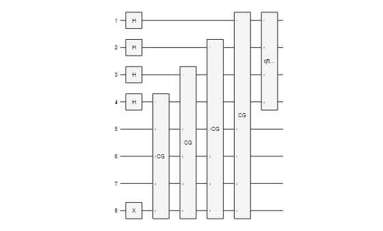
You can implement step 2 in Shor's algorithm by using a quantum phase estimation circuit with $\mathit{n}$ upper qubits and $\mathit{m}$ lower qubits. The circuit consists of the oracle ${\mathit{U}}_{\mathit{f}}$ to handle the modular exponentiation $f\left(x\right)={\mathit{a}}^{\mathit{x}}\mathrm{mod}\mathit{N}$ and the inverse quantum Fourier transform to find the period $\mathit{r}$ from phase estimation, as illustrated in this figure.

The quantum circuit implementation of the modular exponentiation function is a bottleneck in Shor's algorithm. Often, such circuits require a large number of gates, circuit depth, and qubits, which can lead to significant noise and decoherence in the measurement results. However, there are several approaches for constructing the modular exponentiation function (see [2] and [3]). One approach is to use a specially designed circuit for the modular exponentiation function with specific values of $\mathit{a}$ and $\mathit{N}$, as discussed in [3]. This example shows how to implement these specially designed circuits to find the prime factors of 15, 143, and 247 using local simulation.

Create Circuit for Modular Exponentiation

You can decompose the modular exponentiation function $f\left(x\right)={\mathit{a}}^{\mathit{x}}\mathrm{mod}\mathit{N}$ into a product

${\mathit{a}}^{\mathit{x}}\mathrm{mod}\mathit{N}=\left(\dots \left(\left({\mathit{a}}^{{\mathit{x}}_{\mathit{n}}\cdot 2^0}\mathrm{mod}\mathit{N}\right)\times {\mathit{a}}^{{\mathit{x}}_{\mathit{n}-1}\cdot 2^1}\mathrm{mod}\mathit{N}\right)\times \dots \right)\times {\mathit{a}}^{{\mathit{x}}_1\cdot 2^{\mathit{n}-1}}\mathrm{mod}\mathit{N}$,

where

$$\mathit{x}={\mathit{x}}_1\cdot 2^{\mathit{n}-1}+{\mathit{x}}_2\cdot 2^{\mathit{n}-2}+\dots +{\mathit{x}}_{\mathit{n}-1}\cdot 2^1+{\mathit{x}}_{\mathit{n}}\cdot 2^0$$

and $\left|\mathit{x}\right.anglebracketright=\left|{\mathit{x}}_1{\mathit{x}}_2\dots {\mathit{x}}_{\mathit{n}}\right.anglebracketright$ is the binary representation of the variable $\mathit{x}$.

Using this decomposition, the oracle ${\mathit{U}}_{\mathit{f}}$ can be broken down into smaller circuits that perform the controlled operations ${\mathit{a}}^{{\mathit{x}}_{\mathit{i}}\cdot 2^{\mathit{n}-\mathit{i}}}\mathrm{mod}\mathit{N}$ recursively, where ${\mathit{x}}_{\mathit{i}}$ is the state of the $\mathit{i}$th control qubit in the upper register. To decompose the oracle into smaller circuits, apply the modular exponentiation operator ${\mathit{U}}_{\mathit{a}}\left|\mathit{w}\right.anglebracketright=\left|\mathit{w}\cdot \mathit{a}\left(\mathrm{mod}\mathit{N}\right)\right.anglebracketright$ for $2^{\mathit{n}-\mathit{i}}$ times on the state $\left|\mathit{w}\right.anglebracketright$ in the lower register, whose initial state is $\left|0\dots 1\right.anglebracketright$, conditioned on the binary value of ${\mathit{x}}_{\mathit{i}}$.

This figure illustrates the oracle ${\mathit{U}}_{\mathit{f}}$ for the modular exponentiation $\mathit{f}\left(\mathit{x}\right)=7^{\mathit{x}}\mathrm{mod}15$, where $\mathit{n}$ upper qubits represent $\left|\mathit{x}\right.anglebracketright$ and $\mathit{m}$ lower qubits represent $\left|7^{\mathit{x}}\mathrm{mod}15\right.anglebracketright$.

MATLAB® Support Package for Quantum Computing uses a qubit convention that follows most textbooks (see [4]), which is different from the qubit convention in [3]. For a quantum circuit with $\mathit{n}$ qubits, the overall $2^{\mathit{n}}$ basis states are constructed from the Kronecker product of the $\mathit{n}$ qubit bases, ordered from left to right starting with the lowest-index qubit (topmost in the circuit diagram) to the highest-index qubit (bottommost in the circuit diagram). In other words, if the basis of a single qubit with index $\mathit{k}$ is labeled as $\left|{\mathit{q}}_{\mathit{k}}\right.anglebracketright$, which can be $\left|0\right.anglebracketright$ or $\left|1\right.anglebracketright$, then the basis states of the circuit with $\mathit{n}$ qubits are represented by $\left|{\mathit{q}}_1\right.anglebracketright\otimes \dots \left|{\mathit{q}}_{\mathit{k}}\right.anglebracketright\otimes \dots \left|{\mathit{q}}_{\mathit{n}}\right.anglebracketright$. For example, for a circuit with two qubits, all possible basis states expressed as a column vector are $\left|{\mathit{q}}_1{\mathit{q}}_2\right.anglebracketright={\left[\left|00\right.anglebracketright,\left|01\right.anglebracketright,\left|10\right.anglebracketright,\left|11\right.anglebracketright\right]}^{\mathit{T}}$. In contrast, the qubit convention in [3] orders the qubit bases from right to left starting with lowest-index qubit to the highest-index qubit.

Before constructing the oracle ${\mathit{U}}_{\mathit{f}}$, first define a function that creates the controlled-swap gate (CSWAP gate or Fredkin gate). Use the compositeGate function to construct a composite gate from an inner quantum circuit that performs the controlled-swap operation on an outer circuit. Here, qubit 1 is the control qubit, while qubits 2 and 3 are the target qubits to swap in the inner quantum circuit gates. The second input of compositeGate defines the mapping of the qubits of the inner circuit to the qubits of the outer circuit.

function cg = cswapGate(control,target1,target2)
  gates = [cxGate(3,2); ccxGate(1,2,3); cxGate(3,2)];
  cg = compositeGate(gates,[control target1 target2]);
end

Next, define a function that constructs the circuit for the controlled-modular operation $\mathit{a}\mathrm{mod}\mathit{N}$ based on [2] and[3]. In this example, all possible values of $\mathit{a}$ are considered for $\mathit{N}=15$. However, only $\mathit{a}=21$ is considered for $\mathit{N}=143$ and $\mathit{a}=8$ is considered for $\mathit{N}=247$. The first qubit in the inner circuit is set as the control qubit, which is mapped to the $\mathit{i}$th control qubit in the outer circuit that represents the state ${\mathit{x}}_{\mathit{i}}$.

function Ua = modexpUnitary(a,N)
% Construct a mod N based on these references:
% [1] Shor, P. https://doi.org/10.48550/arXiv.quant-ph/9508027.
% [2] Markov, I. L., and M. Saeedi. https://doi.org/10.48550/arXiv.1202.6614.
% [3] Tomčala, J. https://doi.org/10.1007/s10773-023-05532-4.
% For N = 15, the values for a are 2, 4, 7, 8, 11, 13.
% For N = 143, only a = 21 is considered.
% For N = 147, only a = 8 is considered.
% Qubit 1 is set as a control qubit, followed by m qubits as targets.

  % For N = 15, see figure 3 of [2]
  if N == 15
    switch a
      case 2
        Ua = [cswapGate(1,2,5); cswapGate(1,2,3); cswapGate(1,3,4)];
      case 4
        Ua = [cswapGate(1,2,4); cswapGate(1,3,5)];
      case 7
        Ua = [cxGate(1,2:5); cswapGate(1,3,4); cswapGate(1,2,3); cswapGate(1,2,5)];
      case 8
        Ua = [cswapGate(1,2,3); cswapGate(1,2,4); cswapGate(1,2,5)];
      case 11
        Ua = [cxGate(1,2:5); cswapGate(1,2,4); cswapGate(1,3,5)];
      case 13
        Ua = [cxGate(1,2:5); cswapGate(1,2,5); cswapGate(1,2,3); cswapGate(1,3,4)];
    end
  end

  % For N = 143, see figure 8 of [3]
  if N == 143
    switch a
      case 21
        Ua = [mcxGate([1 9],5,[]); mcxGate([1 9],7,[]); cxGate(1,5); ...
              mcxGate([1 5],6,[]); mcxGate([1 5],7,[]); mcxGate([1 5],9,[]); ...
              mcxGate([1 5 9],3,[]); mcxGate([1 5 9],4,[]); mcxGate([1 5 9],6,[]); ...
              mcxGate([1 5 9],7,[]); cxGate(1,[5 7]); mcxGate([1 5 6],3,[]); ...
              mcxGate([1 5 6],4,[]); mcxGate([1 7 9],5,[]); mcxGate([1 7 9],6,[]); ...
              cxGate(1,7)];
    end
  end

  % For N = 247, see figure 6 of [3]
  if N == 247
    switch a
      case 8
        Ua = [cswapGate(1,3,6); cswapGate(1,6,9); cswapGate(1,8,9); ccxGate(1,8,5); ...
              cswapGate(1,2,9); mcxGate([1 5 9],2,[]); mcxGate([1 5 9],4,[]); ...
              cswapGate(1,7,9); mcxGate([1 2 4],5,[]); mcxGate([1 7 9],6,[]); ...
              mcxGate([1 6 7],3,[]); mcxGate([1 6 7],4,[]); mcxGate([1 6 8],9,[]); ...
              mcxGate([1 3 5],4,[]); mcxGate([1 2 3],4,[]); mcxGate([1 2 3],5,[]); ...
              mcxGate([1 2 3],6,[]); mcxGate([1 2 3],9,[]); mcxGate([1 7 8],2,[]); ...
              mcxGate([1 7 8],4,[]); mcxGate([1 7 8],6,[]); cxGate(1,8); ...
              mcxGate([1 5 7 8],2,[]); mcxGate([1 5 7 8],3,[]); ...
              mcxGate([1 5 7 8],4,[]); mcxGate([1 5 7 8],6,[]); ...
              mcxGate([1 5 7 8],9,[]); cxGate(1,8:9); mcxGate([1 7 8 9],2,[]); ...
              mcxGate([1 7 8 9],5,[]); mcxGate([1 7 8 9],6,[]); cxGate(1,9); ...
              mcxGate([1 6 7 8],9,[]); cxGate(1,5:6); mcxGate([1 2 3 6],9,[]); ...
              mcxGate([1 5 6 9],2,[]); mcxGate([1 5 6 9],3,[]); cxGate(1,5:6)];
    end
  end
end

To check the modular exponentiation circuit, you can simulate the circuit and confirm that it satisfies the truth tables for specific input states. For example, the truth table for the operation $7\mathrm{mod}15$ applied repeatedly to an initial input of $0001$ is shown in this table.

${\mathit{U}}_{\mathit{a}}\left|\mathit{w}\right.anglebracketright=\left|\mathit{w}\cdot \mathrm{7}\left(\mathrm{mod}15\right)\right.anglebracketright$in Binary Representation	${\mathit{U}}_{\mathit{a}}\left|\mathit{w}\right.anglebracketright=\left|\mathit{w}\cdot \mathrm{7}\left(\mathrm{mod}15\right)\right.anglebracketright$in Decimal Representation
$${\mathit{U}}_{\mathit{a}}\left|0001\right.anglebracketright=\left|0111\right.anglebracketright$$	$${\mathit{U}}_{\mathit{a}}\left|1\right.anglebracketright\to \left|7\right.anglebracketright$$
$${\mathit{U}}_{\mathit{a}}\left|0111\right.anglebracketright=\left|0100\right.anglebracketright$$	$${\mathit{U}}_{\mathit{a}}\left|7\right.anglebracketright\to \left|4\right.anglebracketright$$
$${\mathit{U}}_{\mathit{a}}\left|0100\right.anglebracketright=\left|1101\right.anglebracketright$$	$${\mathit{U}}_{\mathit{a}}\left|4\right.anglebracketright\to \left|13\right.anglebracketright$$
$${\mathit{U}}_{\mathit{a}}\left|1101\right.anglebracketright=\left|0001\right.anglebracketright$$	$${\mathit{U}}_{\mathit{a}}\left|13\right.anglebracketright\to \left|1\right.anglebracketright$$
$${\mathit{U}}_{\mathit{a}}\left|0001\right.anglebracketright=\left|0111\right.anglebracketright$$	${\mathit{U}}_{\mathit{a}}\left|1\right.anglebracketright\to \left|7\right.anglebracketright$

Use the modexpUnitary function to construct the circuit for the controlled-modular operation $7\mathrm{mod}15$. Specify an initial state of $1$ for the control qubit, such that the condition to apply ${\mathit{U}}_{\mathit{a}}$ is always true, and initialize the state of the lower $\mathit{m}$ qubits as $0001$. Here, because the ${\mathit{U}}_{\mathit{a}}$ operation result can never exceed $\mathit{N}-1$, using $\mathit{m}=4$ qubits is adequate for $\mathit{N}=15$.

N = 15;
a = 7;
m = 4;
Ua = modexpUnitary(a,N);
initState = "1" + string(dec2bin(1,m))

initState = 
"10001"

Construct the modular exponentiation circuit to check against the truth table by using compositeGate to apply the operation $7\mathrm{mod}15$ recursively. Simulate the output state of this circuit and show the result in binary and decimal representations. The circuit simulation results match the truth tables.

gates = compositeGate(Ua,[1 2:(m+1)]);
c = quantumCircuit(gates);
state = initState;
for k = 1:5
  state = simulate(c,state);
  bitStr = char(formula(state))
  dec = bin2dec(bitStr(end-m:end-1))
end

bitStr = 
'1 * |10111>'

dec = 
7

bitStr = 
'1 * |10100>'

dec = 
4

bitStr = 
'1 * |11101>'

dec = 
13

bitStr = 
'1 * |10001>'

dec = 
1

bitStr = 
'1 * |10111>'

dec = 
7

Find Prime Factors of 15

Define the composite number $\mathit{N}$ to factor.

N = 15

N = 
15

Define a function that finds the integers $1<a<N$ that are coprime to $\mathit{N}$.

function aList = findCoprime(n)
  aList = [];
  for x = 2:(n-1)
    if gcd(x,n) == 1
      aList(end+1) = x;
    end
  end
end

Choose an integer $\mathit{a}$ from the list of integers that the findCoprime function returns. For this example, choose the third integer in the list.

aList = findCoprime(N);
a = aList(3)

a = 
7

Next, define the number of qubits. The first register of the upper qubits $\mathit{n}$ determines the accuracy of the phase estimation. A higher number of these qubits results in a more accurate detection of the period searched, but it also increases the depth of the whole circuit. For this example, choosing $\mathit{n}=4$ is adequate to find the prime factors of 15. The second register of the lower qubits $\mathit{m}$ determines the binary representation of the modular exponentiation ${\mathit{a}}^{\mathit{x}}\mathrm{mod}\mathit{N}$, which can be selected using $\mathit{m}=\lceil {\log }_2\left(\mathit{N}-1\right)\rceil$.

n = 4;
m = ceil(log2(N-1));

Construct the oracle ${\mathit{U}}_{\mathit{f}}$ that finds the modular exponentiation $f\left(x\right)={\mathit{a}}^{\mathit{x}}\mathrm{mod}\mathit{N}$. Create the modular exponentiation gates for the oracle in a loop, and map their qubits to the qubits of the outer circuit.

UfQPE = [];
for k = 0:n-1
  Ua_2tok = compositeGate(repmat(modexpUnitary(a,N),2^k,1), ...
                          [n-k (n+1):(n+m)]);
  UfQPE = [UfQPE; Ua_2tok];
end

Construct the whole quantum phase estimation circuit. Then plot the circuit.

gates = [hGate(1:n); xGate(n+m)];
gates = [gates; UfQPE; inv(qftGate(1:n))];
c = quantumCircuit(gates);
figure
plot(c)

Simulate the circuit. Show the histogram of the possible states of the upper register with a probability threshold of 0.02.

s = simulate(c);
histogram(s,1:n,Threshold=0.02)

To return these possible states and the probability of measuring each state, use querystates. Specify the probability threshold as 0.02. The possible states are returned as binary representations.

[states,probabilities] = querystates(s,1:n,Threshold=0.02);

Convert these binary states into decimal form, which represents the phase estimation.

phase = bin2dec(states)/2^n

phase = 4×1

         0
    0.2500
    0.5000
    0.7500

Determine the period of the phase using continued fraction or rational fraction approximation. Use the rat function and specify the tolerance as 1/2 of the smallest interval spacing between the converted phases, which is $1/2^{\mathit{n}+1}$. The returned values in den represent possible values of the period $\mathit{r}$.

[num,den] = rat(phase,1/2^(n+1))

num = 4×1

     0
     1
     1
     3

den = 4×1

     1
     4
     2
     4

Next, from the denominators of the continued fractions, check if the period $\mathit{r}$ is even and if it satisfies the relation ${\mathit{a}}^{\mathit{r}/2}\not\equiv -1\left(\mathrm{mod}\mathit{N}\right)$. If both conditions are true, then compute the prime factors of $\mathit{N}$.

found = false;
attempt = 1;
while ~found && attempt <= numel(den)
  r = den(attempt);
  if mod(r,2) == 0 && phase(attempt) ~= 0
      p = gcd(a^(floor(r/2))-1,N);
      q = gcd(a^(floor(r/2))+1,N);
      found = true;
  else
    attempt = attempt + 1;
  end
end
if found == true
  fprintf("Prime factors found: %d and %d \n", p, q);
else
  fprintf("No factors found. Choose different a.")
end

Prime factors found: 3 and 5 

Find Prime Factors of 143 and 247

Find the prime factors of 143 and 247. Here, the initial guess for $\mathit{a}$ is predetermined based on the specially designed circuit for the modular exponentiation operation, as discussed in [3]. Define a function findPrimeFactors that reuses the code in the previous section. Here, choosing $\mathit{n}=7$ is adequate to find the prime factors of 143 and 247.

function [p,q] = findPrimeFactors(N,a)
  n = 7;
  m = ceil(log2(N-1));
  UfQPE = [];
  for k = 0:n-1
    Ua_2tok = compositeGate(repmat(modexpUnitary(a,N),2^k,1), ...
                            [n-k (n+1):(n+m)]);
    UfQPE = [UfQPE; Ua_2tok];
  end
  gates = [hGate(1:n); xGate(n+m)];
  gates = [gates; UfQPE; inv(qftGate(1:n))];
  c = quantumCircuit(gates);
  s = simulate(c);
  [states,probabilities] = querystates(s,1:n,Threshold=0.02);
  phase = bin2dec(states)/2^n;
  [num,den] = rat(phase,1/2^(n+1));
  found = false;
  attempt = 1;
  while ~found && attempt <= numel(den)
    r = den(attempt);
    if mod(r,2) == 0 && phase(attempt) ~= 0
      p = gcd(a^(floor(r/2))-1,N);
      q = gcd(a^(floor(r/2))+1,N);
      found = true;
    else
      attempt = attempt + 1;
    end
  end
  if found == true
    fprintf("Prime factors found: %d and %d \n", p, q);
  else
    p = 1;
    q = N;
    fprintf("No factors found. Choose different a.")
  end
end

Find the prime factors of 143 by choosing $\mathit{a}$ as 21.

[p,q] = findPrimeFactors(143,21)

Prime factors found: 11 and 13 

p = 
11

q = 
13

Find the prime factors of 247 by choosing $\mathit{a}$ as 8.

[p,q] = findPrimeFactors(247,8)

Prime factors found: 19 and 13 

p = 
19

q = 
13

References

[1] Shor, Peter W. "Polynomial-Time Algorithms for Prime Factorization and Discrete Logarithms on a Quantum Computer." arXiv, January 25, 1996. https://doi.org/10.48550/arXiv.quant-ph/9508027.

[2] Markov, Igor L., and Mehdi Saeedi. "Constant-Optimized Quantum Circuits for Modular Multiplication and Exponentiation." arXiv, April 2, 2015. https://doi.org/10.48550/arXiv.1202.6614.

[3] Tomčala, J. "On the Various Ways of Quantum Implementation of the Modular Exponentiation Function for Shor's Factorization." International Journal of Theoretical Physics 63, no. 1 (January 10,2024): 14. https://doi.org/10.1007/s10773-023-05532-4.

[4] Singleton Jr, Robert L. "Shor's Factoring Algorithm and Modular Exponentiation Operators." Quanta 12, no. 1 (September 15, 2023): 41–130. https://doi.org/10.12743/quanta.v12i1.235.