spectralMatch

Identify unknown regions or materials using spectral library

Since R2020a

Syntax

score = spectralMatch(libData,hcube)

score = spectralMatch(libData,reflectance,wavelength)

score = spectralMatch(___,Name,Value)

Description

score = spectralMatch(libData,hcube) identifies regions in a hyperspectral data cube by matching spectra signature of each pixel to the spectral data read from the ECOSTRESS spectral library libData.

score = spectralMatch(libData,reflectance,wavelength) identifies a region or material by matching its spectral reflectance values, specified as reflectance and wavelength, with the values available in the ECOSTRESS spectral library libData.

score = spectralMatch(___,Name,Value) specifies options using one or more name-value pair arguments in addition to any combination of input arguments in previous syntaxes.

Note

This function requires the Image Processing Toolbox™ Hyperspectral Imaging Library. You can install the Image Processing Toolbox Hyperspectral Imaging Library from Add-On Explorer. For more information about installing add-ons, see Get and Manage Add-Ons.

The Image Processing Toolbox Hyperspectral Imaging Library requires desktop MATLAB^®, as MATLAB Online™ or MATLAB Mobile™ do not support the library.

Examples

Segment Vegetation Regions in Hyperspectral Data Using Spectral Matching

The spectral matching method compares the spectral signature of each pixel in the hyperspectral data cube with a reference spectral signature for vegetation from an ECOSTRESS spectrum file.

Read the spectral signature of vegetation from the ECOSTRESS spectral library.

fileroot = matlabshared.supportpkg.getSupportPackageRoot();
filename = fullfile(fileroot,'toolbox','images','supportpackages','hyperspectral','hyperdata',...
               'ECOSTRESSSpectraFiles','vegetation.tree.tsuga.canadensis.vswir.tsca-1-47.ucsb.asd.spectrum.txt');
libData = readEcostressSig(filename);

Read the hyperspectral data into the workspace.

hcube = hypercube('paviaU.hdr');

Compute the distance scores of the spectrum of the hyperspectral data pixels with respect to the reference spectrum.

score = spectralMatch(libData,hcube);

Display the distance scores. The pixels with low distance scores are stronger matches to the reference spectrum and are more likely to belong to the vegetation region.

figure
imagesc(score)
colorbar

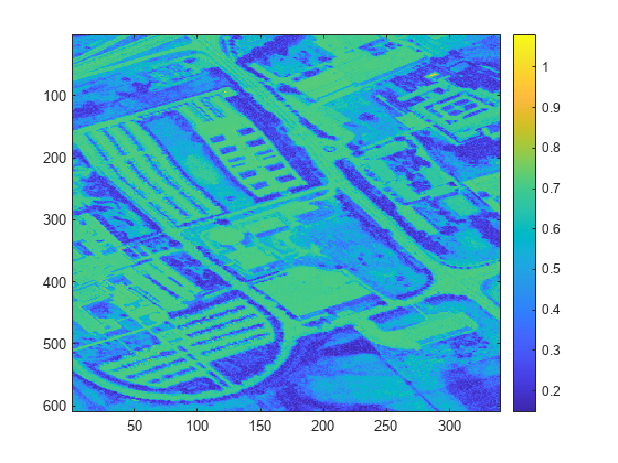
Define a threshold for detecting distance scores that correspond to the vegetation region.

threshold = 0.3;

Generate a binary image by assigning a intensity value 1 for pixels with score less than a specified threshold. Other regions are assigned the intensity value 0. The maximum intensity regions in the binary image correspond to the vegetation regions in the hyperspectral data cube.

bw = score < threshold;

Segment the vegetation regions of the hyperspectral data cube by using the indices of the maximum intensity regions in the binary image.

T = reshape(hcube.DataCube,[size(hcube.DataCube,1)*size(hcube.DataCube,2) size(hcube.DataCube,3)]);
Ts = zeros(size(T));
Ts(bw == 1,:) = T( bw==1 ,:);
Ts = reshape(Ts,[size(hcube.DataCube,1) size(hcube.DataCube,2) size(hcube.DataCube,3)]);

. Create a new hypercube object that contains only the segmented vegetation regions.

segmentedDataCube = hypercube(Ts,hcube.Wavelength);

Estimate the RGB colour image of the original data cube and the segmented data cube by using the colorize function.

rgbImg = colorize(hcube,'Method','rgb','ContrastStretching',true);
segmentedImg = colorize(segmentedDataCube,'Method','rgb','ContrastStretching',true);

Overlay the binary image on the RGB version of the original data cube by using the imoverlay function.

B = imoverlay(rgbImg,bw,'Yellow');

Display the RGB colour images of the original data cube and the segmented data cube along with the overlaid image. The segmented image contains only the vegetation regions that are segmented from the original data cube.

figure
montage({rgbImg segmentedImg B},'Size',[1 3])
title(['Original Image | ' 'Segmented Image | ' 'Overlayed Image'])

Identify Unknown Spectral Signature Using Spectral Matching

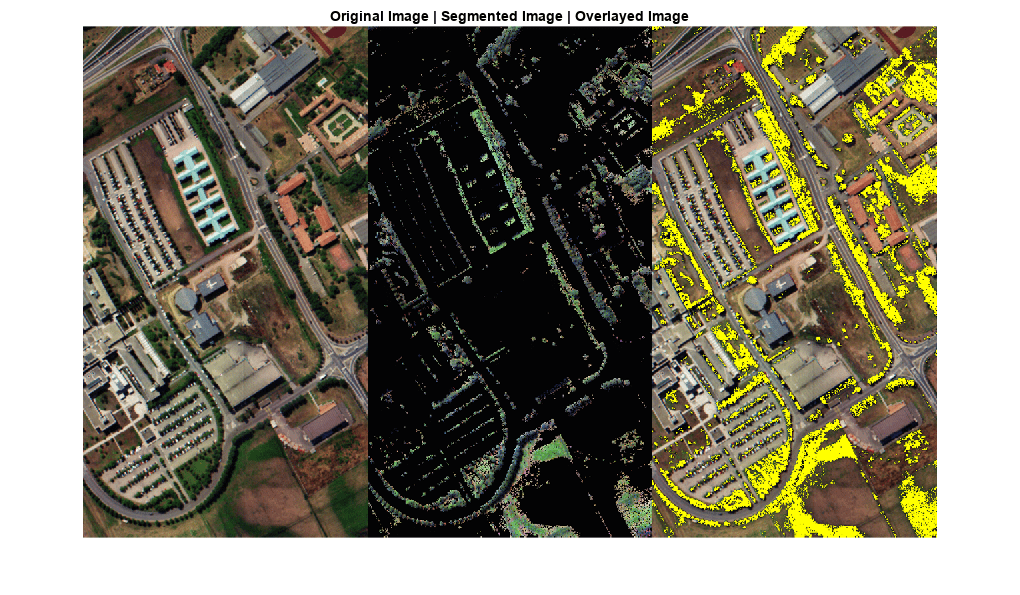
Read reference spectral signatures from the ECOSTRESS spectral library. The library consists of 15 spectral signatures belonging to manmade materials, soil, water, and vegetation. The output is a structure array that stores the spectral data read from ECOSTRESS library files.

fileroot = matlabshared.supportpkg.getSupportPackageRoot();
dirname = fullfile(fileroot,'toolbox','images','supportpackages','hyperspectral','hyperdata','ECOSTRESSSpectraFiles');
libData = readEcostressSig(dirname);

Load a .mat file that contains the reflectance and the wavelength values of an unknown material into the workspace. The reflectance and the wavelength values together comprise the test spectrum.

load spectralData 'reflectance' 'wavelength'

Compute the spectral match between the reference spectrum and test spectrum using spectral information divergence (SID) method. The function computes the distance score for only those reference spectra that have bandwidth overlap with the test spectrum. The function displays a warning message for all other spectra.

score = spectralMatch(libData,reflectance,wavelength,'Method','SID');

Warning: Unable to find overlapping wavelengths between test spectra and library signature number 8

Warning: Unable to find overlapping wavelengths between test spectra and library signature number 9

Warning: Unable to find overlapping wavelengths between test spectra and library signature number 11

Display the distance scores of the test spectrum. The pixels with lower distance scores are stronger matches to the reference spectrum. A distance score value of NaN indicates that the corresponding reference spectrum and the test spectrum do not meet the overlap bandwidth threshold.

score

score = 1×15

  297.8016  122.5567  203.5864  103.3351  288.7747  275.5321  294.2341       NaN       NaN  290.4887       NaN  299.5762  171.6919   46.2072  176.6637

Find the minimum distance score and the corresponding index. The returned index value indicates the row of the structure array libData that contains the reference spectrum that most closely matches a test spectrum.

[value,ind] = min(score);

Find the matching reference spectrum by using the index of the minimum distance score, and display the details of the matching spectral data in the ECOSTRESS library. The result shows that the test spectrum match most closely with the spectral signature of sea water.

matchingSpectra = libData(ind)

matchingSpectra = struct with fields:
                     Name: "Sea Foam"
                     Type: "Water"
                    Class: "Sea Water"
                 SubClass: "none"
             ParticleSize: "Liquid"
                    Genus: [0×0 string]
                  Species: [0×0 string]
                 SampleNo: "seafoam"
                    Owner: "Dept. of Earth and Planetary Science, John Hopkins University"
          WavelengthRange: "TIR"
                   Origin: "JHU IR Spectroscopy Lab."
           CollectionDate: "N/A"
              Description: "Sea foam water. Original filename FOAM Original ASTER Spectral Library name was jhu.becknic.water.sea.none.liquid.seafoam.spectrum.txt"
              Measurement: "Directional (10 Degree) Hemispherical Reflectance"
              FirstColumn: "X"
             SecondColumn: "Y"
           WavelengthUnit: "micrometer"
                 DataUnit: "Reflectance (percent)"
              FirstXValue: "14.0112"
               LastXValue: "2.0795"
          NumberOfXValues: "2110"
    AdditionalInformation: "none"
               Wavelength: [2110×1 double]
              Reflectance: [2110×1 double]

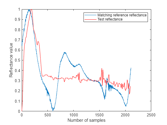
Plot the reflectance values of the test spectrum and the corresponding reference spectrum. For the purpose of plotting and visualizing the shape of the reflectance curves, rescale the reflectance values to the range [0, 1] and interpolate test reflectance values to match the reference reflectance values in number.

figure
testReflectance = rescale(reflectance,0,1);
refReflectance = rescale(matchingSpectra.Reflectance,0,1);
testLength = length(testReflectance);
newLength = length(testReflectance)/length(refReflectance);
testReflectance = interp1(1:testLength,testReflectance,1:newLength:testLength);

plot(refReflectance)
hold on
plot(testReflectance,'r')
hold off
legend('Matching reference reflectance','Test reflectance')
xlabel('Number of samples')
ylabel('Reflectance value')

Input Arguments

libData — ECOSTRESS Spectral data

structure

Spectral data from ECOSTRESS files, returned as a 1-by-K structure array. K is the number of spectrum files read by the function. Each element of the structure array has 24 fields that contain the header information of the spectrum files.

Field Names	Description
Name	Name of the measured sample or material
Type	Type of sample, such as "mineral", "rock", "tree", or "manmade"
Class	Class of the sample type For example, if the sample type is "mineral" then the class can be: "native elements","silicates", "oxides", "sulfides", "sulfates", "halides", "carbonates", "phosphates", or "mineraloids".
SubClass	Subclass of the sample type This field contains an empty array or "none", unless the Type value is "mineral", "rock", "manmade", "soil", "lunar", or "meteorite".
ParticleSize	Particle size of the sample type This field contains an empty array unless the Type value is "mineral", "rock", "manmade", "soil", "lunar", or "meteorite".
Genus	Genus of the sample This field contains an empty array unless the Type value is "vegetation" or "nonphotosynthetic".
Species	Species of the sample This field contains an empty array unless the Type value is "vegetation" or "nonphotosynthetic".
SampleNo	Sample number This value is an identifier for the associated sample.
Owner	Owner of the sample
WavelengthRange	Wavelength range of the measured sample The value must be "All", "TIR", or "VSWIR".
Origin	Location from which the data was obtained
CollectionDate	Date on which the sample was collected This value is in mm/dd/yy format.
Description	Description of the measured sample This field provides additional information about the characteristics of the sample.
Measurement	Spectral measurement mode used to measure the sample
FirstColumn	First column of data values in the spectrum file
SecondColumn	Second column of data values in the spectrum file
WavelengthUnit	Measuring unit for the spectral wavelengths of the samples The value for every sample type is "micrometer". This field corresponds to the X Units field of the header data in the ECOSTRESS spectrum file.
DataUnit	Unit of the spectral measurement mode Spectral measurement mode includes reflectance, transmittance, and transmission. The unit is percentage. This field corresponds to the Y Units field of the header data in the ECOSTRESS spectrum file.
FirstXValue	First value in the first column of data values in the spectrum file
LastXValue	Last value in the first column of data values in the spectrum file
NumberofXValues	Total number of data values in the first column of the spectrum file
AdditionalInformation	Additional information about the sample This field includes information that is not part of the spectral data.
Wavelength	Wavelength values at which the reflectances were measured
Reflectance	Reflectance values measured at each wavelengths

hcube — Input hyperspectral data

hypercube object

Input hyperspectral data, specified as a hypercube object. The DataCube property of the hypercube object contains the hyperspectral datacube.

reflectance — Reflectance values

C-element vector

Reflectance values, specified as a C-element vector. C is the number of wavelengths for which the reflectance values have been measured.

wavelength — Wavelength values

C-element vector

Wavelength values, specified as a C-element vector. C is the number of wavelengths for which the reflectance values have been measured.

Name-Value Arguments

Specify optional pairs of arguments as Name1=Value1,...,NameN=ValueN, where Name is the argument name and Value is the corresponding value. Name-value arguments must appear after other arguments, but the order of the pairs does not matter.

Before R2021a, use commas to separate each name and value, and enclose Name in quotes.

Example: spectralMatch(libData,hcube,'MinBandWidth',0.5)

Method — Spectral matching method

'sam' (default) | 'sid' | 'sidsam' | 'jmsam' | 'ns3'

Spectral matching method, specified as the comma-separated pair consisting of 'Method' and one of these values:

• 'sam' — Spectral angle mapper (SAM) method, which measures the similarity between two spectra by computing the angular distance between them.

• 'sid' — Spectral information divergence (SID) method, which measures the similarity between two spectra by computing the difference between their probability distribution values.

• 'sidsam' — Mixed spectral similarity method, which measures the similarity between two spectra by combining the SID and SAM distance measures.

• 'jmsam' — Jeffries Matusita-Spectral Angle Mapper (JMSAM), which measures the similarity between two spectra by combining the Jeffries Matusita (JM) and SAM distance measures.

• 'ns3' — Normalized spectral similarity score (NS3) method, which measures the similarity between two spectra by combining the Euclidean and SAM distance measures.

For details about these spectral matching methods, see More About.

Data Types: char | string

MinBandWidth — Minimum overlap bandwidth

300 (default) | positive scalar

Minimum overlap bandwidth, specified as the comma-separated pair consisting of 'MinBandWidth' and a positive scalar in nanometers. The overlap bandwidth between the reference spectrum and the test spectra is defined as:

BW_overlap = W_max − W_min

W_min is the maximum of minimum wavelengths in the reference and test spectra.

W_max is the maximum of maximum wavelengths in the reference and test spectra.

The 'MinBandWidth' argument defines the minimum expected value for the overlap bandwidth between the spectral values of the test material and the ECOSTRESS spectral data.

Data Types: single | double | int8 | int16 | int32 | int64 | uint8 | uint16 | uint32 | uint64

Output Arguments

score — Distance scores

3-D numeric array | matrix | K-element column vector | scalar

Distance scores, returned as a 3-D numeric array, matrix, K-element column vector, or scalar. The dimensions of the output score depend on the dimensions of the libData and whether the test data is a hypercube object or a wavelength and reflectance pair.

If the test spectral signatures are specified as a hypercube object, hcube and the data cube is of size M-by-N-by-C:

Dimension of input argument, libData	Dimension of output, score
1-by-K, containing K reference signatures read from K number of spectrum files	3-D numeric array of size M-by-N-by-K containing the distance score for each pixel with respect to K reference signatures The values in each channel of K are the distance scores of the spectra of each pixel with respect to the spectral data in the corresponding row of libData. Similarly, the values in the second channel relate to the spectral data in the second row of libData.
1-by-1, containing reference signature read from one spectrum file (K = 1)	matrix of size M-by-N, The matrix contains the distance score for each pixel's spectra with respect to a reference signature.

If the test spectral signature is specified as reflectance and wavelength values:

Dimension of input argument, libData	Dimension of output, score
1-by-K, containing K reference signatures read from K number of spectrum files	K-element vector containing the distance score of the test spectra with respect to K reference signatures. Each element of the vector is the distance score of the test reflectance values with respect to the spectral data in the corresponding row of libData.
1-by-1, containing reference signature read from one spectrum file (K = 1)	scalar

Data Types: double

More About

Spectral Angle Mapper (SAM)

Given the test spectra t and a reference spectra r of length C, the SAM score α is calculated as

$$\alpha ={\cos }^{-1}\left(\frac{{\displaystyle \sum _{i=1}^C{t}_i{r}_i}}{\sqrt{{\displaystyle \sum _{i=1}^C{t}_i^2}}\sqrt{{\displaystyle \sum _{i=1}^C{r}_i^2}}}\right).$$

Spectral Information Divergence (SID)

The spectral information divergence (SID) method computes spectral similarity based on the divergence between the probability distributions of the two spectra. Let r and t be the reference and test spectra respectively. Calculate the distribution values for the reference spectra as:

$$q_i=\frac{r_i}{{\displaystyle \sum _{i=1}^C{r}_i}}.$$

.

Calculate the distribution values for the test spectra as:

$$p_i=\frac{t_i}{{\displaystyle \sum _{i=1}^C{t}_i}}.$$

.

Then, compute the SID value by using the probability distributions of the reference and the test spectra:

$$SID={\displaystyle \sum _{i=1}^C{p}_i\log \left(\frac{p_i}{q_i}\right)+}{\displaystyle \sum _{i=1}^C{q}_i\log \left(\frac{q_i}{p_i}\right)}.$$

SID-SAM

The SID-SAM method computes spectral similarity as:

$$SIDSAM=SID\times \tan \left(\alpha \right)$$

Jeffries Matusita-Spectral Angle Mapper (JMSAM)

The JMSAM method computes spectral similarity based on the Jeffries Matusita (JM) and SAM distances between two spectra. Let r and t be the reference and test spectra respectively.

First, compute the JM distance,

$$J{M}_{\text{distance}}=2\left(1-e^{-B}\right)$$

where B is the Bhattacharyya distance,

$$B=\frac{1}{8}{\left({\mu }_t-{\mu }_r\right)}^T{\left[\frac{{\sigma }_t+{\sigma }_r}{2}\right]}^{-1}\left({\mu }_t-{\mu }_r\right)+\frac{1}{2}\ln \left[\frac{\left|\frac{{\sigma }_t+{\sigma }_r}{2}\right|}{\sqrt{\left|{\sigma }_t\right|\left|{\sigma }_r\right|}}\right]$$

μ_r and μ_t are the mean values of the reference and test spectra respectively. σ_r and σ_t are the covariance values of the reference and test spectra respectively.

Then, compute the SAM value α by using the test spectra t and the reference spectra r of length C,

$$\alpha ={\cos }^{-1}\left(\frac{{\displaystyle \sum _{i=1}^C{t}_i{r}_i}}{\sqrt{{\displaystyle \sum _{i=1}^C{t}_i^2}}\sqrt{{\displaystyle \sum _{i=1}^C{r}_i^2}}}\right).$$

Finally, compute the JMSAM score as:

$$JMSAM=J{M}_{distance}\times \tan \left(\alpha \right)$$

Normalized Spectral Similarity Score (NS3)

The NS3 method computes spectral similarity based on the Euclidean and SAM distances between two spectra. Let r and t be the reference and test spectra respectively. Compute the Euclidean distance between two spectra as:

$$A_{Euclidean}=\sqrt{\frac{1}{C}{\displaystyle \sum _{i=1}^C{\left(t_i-r_i\right)}^2}}$$

Then, compute the SAM value α

$$\alpha ={\cos }^{-1}\left(\frac{{\displaystyle \sum _{i=1}^C{t}_i{r}_i}}{\sqrt{{\displaystyle \sum _{i=1}^C{t}_i^2}}\sqrt{{\displaystyle \sum _{i=1}^C{r}_i^2}}}\right).$$

Finally, compute the NS3 score as:

$$NS3=\sqrt{A_{Euclidean}{}^2+{\left(1-\cos \left(\alpha \right)\right)}^2}$$

Version History

Introduced in R2020a