locallapfilt
Fast local Laplacian filtering of images
Syntax
Description
B = locallapfilt(___,Name=Value)
Examples
Import an RGB image
A = imread('peppers.png');Set parameters of the filter to increase details smaller than 0.4.
sigma = 0.4;
alpha = 0.5;
Use fast local Laplacian filtering
B = locallapfilt(A, sigma, alpha);
Display the original and filtered images side-by-side.
imshowpair(A, B, 'montage')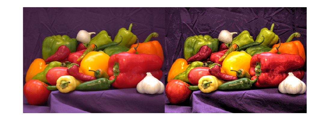
Local Laplacian filtering is a computationally intensive algorithm. To speed up processing, locallapfilt approximates the algorithm by discretizing the intensity range into a number of samples defined by the 'NumIntensityLevels' parameter. This parameter can be used to balance speed and quality.
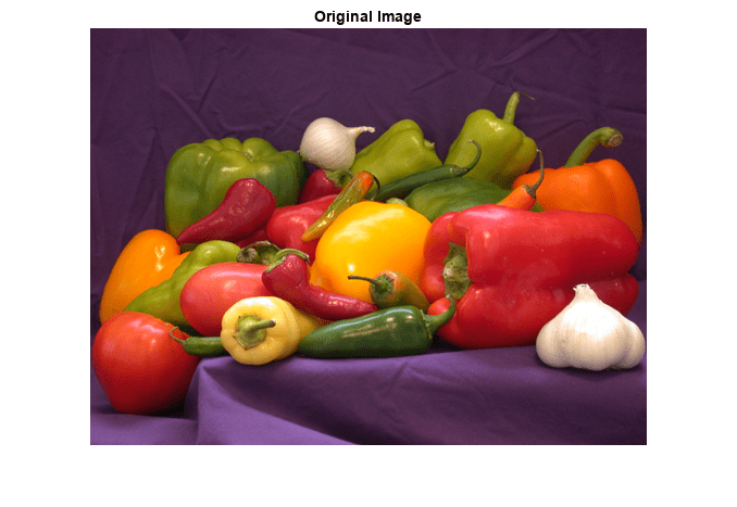
Import an RGB image and display it.
A = imread('peppers.png');
figure
imshow(A)
title('Original Image')
Use a sigma value to process the details and an alpha value to increase the contrast, effectively enhancing the local contrast of the image.
sigma = 0.2;
alpha = 0.3;
Using fewer samples increases the execution speed, but can produce visible artifacts, especially in areas of flat contrast. Time the function using only 20 intensity levels.
t_speed = timeit(@() locallapfilt(A, sigma, alpha, 'NumIntensityLevels', 20)) t_speed = 0.0115
Now, process the image and display it.
B_speed = locallapfilt(A, sigma, alpha, 'NumIntensityLevels', 20);
figure
imshow(B_speed)
title(['Enhanced with 20 intensity levels in ' num2str(t_speed) ' sec'])

A larger number of samples yields better looking results at the expense of more processing time. Time the function using 100 intensity levels.
t_quality = timeit(@() locallapfilt(A, sigma, alpha, 'NumIntensityLevels', 100))t_quality = 0.0337
Process the image with 100 intensity levels and display it:
B_quality = locallapfilt(A, sigma, alpha, 'NumIntensityLevels', 100);
figure
imshow(B_quality)
title(['Enhancement with 100 intensity levels in ' num2str(t_quality) ' sec'])
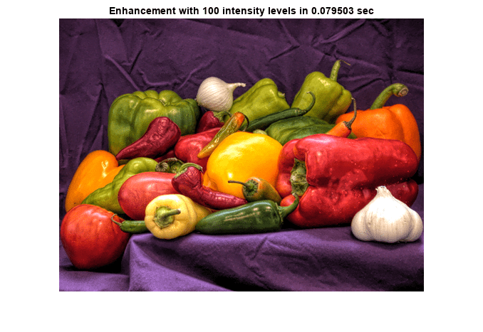
Try varying the number of intensity levels on your own images. Try also flattening the contrast (with alpha > 1). You will see that the optimal number of intensity levels is different for every image and varies with alpha. By default, locallapfilt uses a heuristic to balance speed and quality, but it cannot predict the best value for every image.
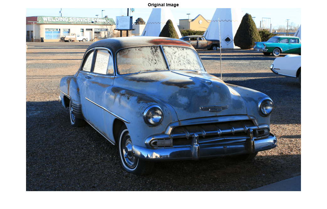
Import a color image, reduce its size, and display it.
A = imread('car2.jpg');
A = imresize(A, 0.25);
figure
imshow(A)
title('Original Image')
Set the parameters of the filter to dramatically increase details smaller than 0.3 (out of a normalized range of 0 to 1).
sigma = 0.3;
alpha = 0.1;
Let's compare the two different modes of color filtering. Process the image by filtering its intensity and by filtering each color channel separately:
B_luminance = locallapfilt(A, sigma, alpha);
B_separate  = locallapfilt(A, sigma, alpha, 'ColorMode', 'separate');
Display the filtered images.
figure
imshow(B_luminance)
title('Enhanced by boosting the local luminance contrast')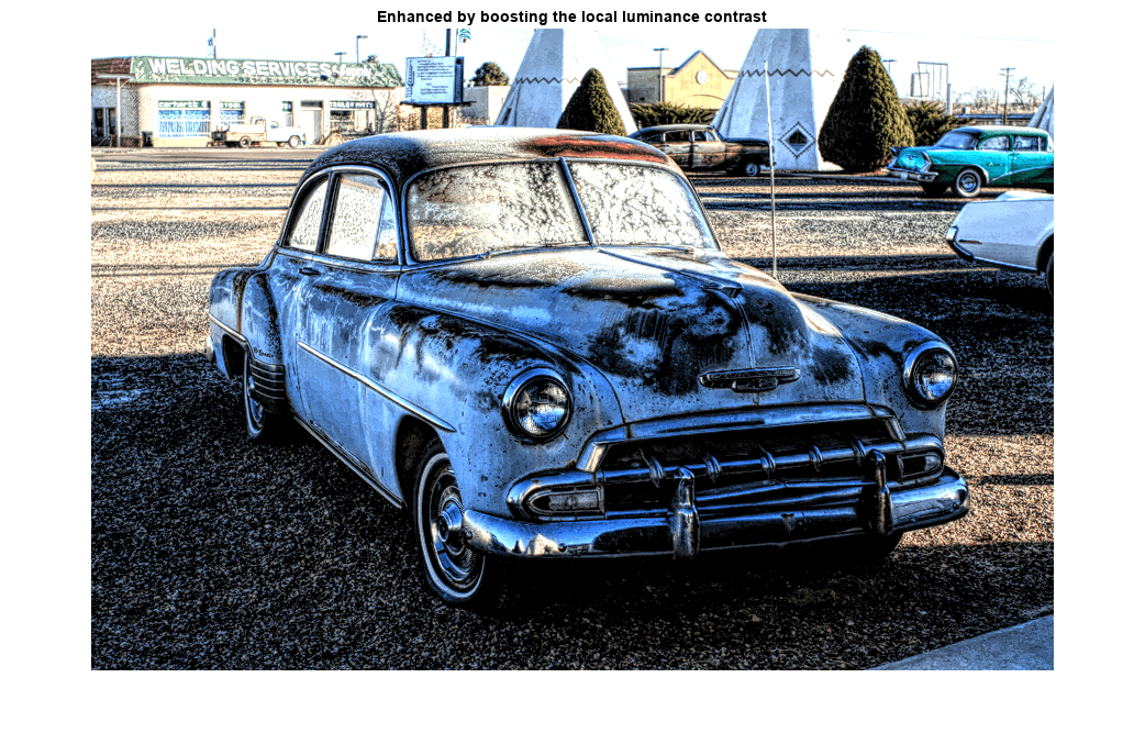
figure
imshow(B_separate)
title('Enhanced by boosting the local color contrast')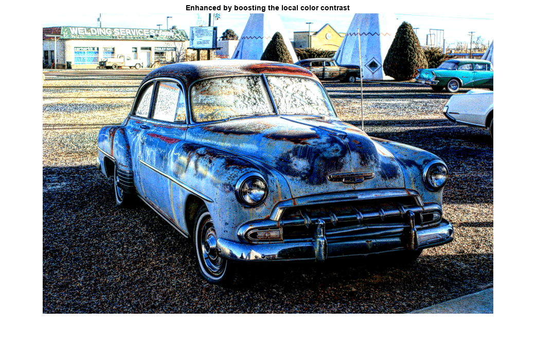
An equal amount of contrast enhancement has been applied to each image, but colors are more saturated when setting 'ColorMode' to 'separate'.
Import an image. Convert the image to floating point so that we can add artificial noise more easily.
A = imread('pout.tif');
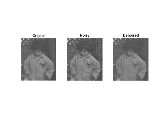
A = im2single(A);Add Gaussian noise with zero mean and 0.001 variance.
A_noisy = imnoise(A, 'gaussian', 0, 0.001);
psnr_noisy = psnr(A_noisy, A);
fprintf('The peak signal-to-noise ratio of the noisy image is %0.4f\n', psnr_noisy);
The peak signal-to-noise ratio of the noisy image is 30.0234
Set the amplitude of the details to smooth, then set the amount of smoothing to apply.
sigma = 0.1;
alpha = 4.0;
Apply the edge-aware filter.
B = locallapfilt(A_noisy, sigma, alpha);
psnr_denoised = psnr(B, A);
fprintf('The peak signal-to-noise ratio of the denoised image is %0.4f\n', psnr_denoised);
The peak signal-to-noise ratio of the denoised image is 32.3362
Note an improvement in the PSNR of the image.
Display all three images side by side. Observe that details are smoothed and sharp intensity variations along edges are unchanged.
figure
subplot(1,3,1), imshow(A), title('Original')
subplot(1,3,2), imshow(A_noisy), title('Noisy')
subplot(1,3,3), imshow(B), title('Denoised')
Import the image, resize it and display it
A = imread('car1.jpg');
A = imresize(A, 0.25);
figure
imshow(A)
title('Original Image')
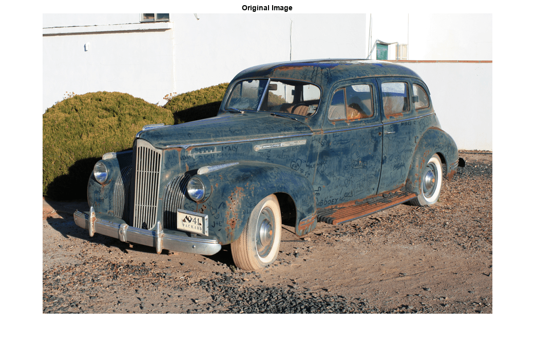
The car is dirty and covered in markings. Let's try to erase the dust and markings on the body. Set the amplitude of the details to smooth, and set a large amount of smoothing to apply.
sigma = 0.2;
alpha = 5.0;
When smoothing (alpha > 1), the filter produces high quality results with a small number of intensity levels. Set a small number of intensity levels to process the image faster.
numLevels = 16;
Apply the filter.
B = locallapfilt(A, sigma, alpha, 'NumIntensityLevels', numLevels);Display the "clean" car.
figure
imshow(B)
title('After smoothing details')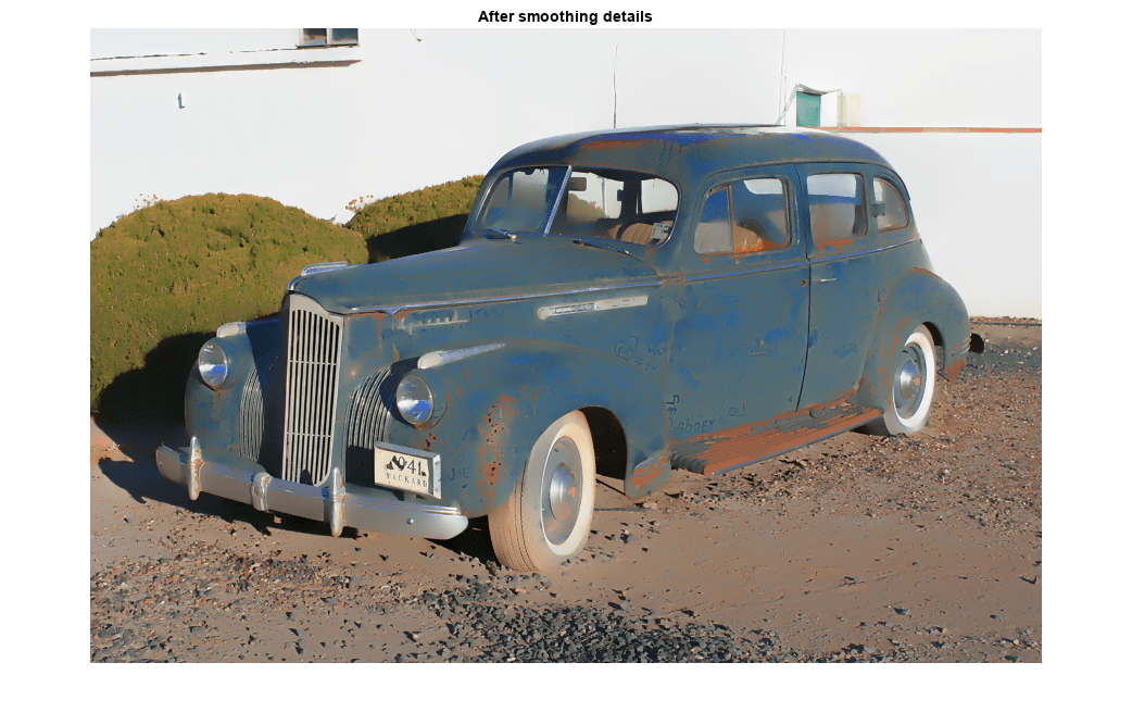
Input Arguments
Name-Value Arguments
Output Arguments
References
[1] Paris, Sylvain, Samuel W. Hasinoff, and Jan Kautz. Local Laplacian filters: edge-aware image processing with a Laplacian pyramid, ACM Trans. Graph. 30.4 (2011): 68.
[2] Aubry, Mathieu, et al. Fast local laplacian filters: Theory and applications. ACM Transactions on Graphics (TOG) 33.5 (2014): 167.