empiricalLine
Empirical line calibration of hyperspectral data
Description
Add-On Required: This feature requires the Hyperspectral Imaging Library for Image Processing Toolbox add-on.
newhcube = empiricalLine(hcube,imgSpectra,fieldSpectra,fieldWL)hcube.
The function calculates empirical line factors to force the image spectral data,
imgSpectra, to match the field reflectance spectra,
fieldSpectra, with wavelengths fieldWL. For more
information, see Algorithms.
Note
The Hyperspectral Imaging Library for Image Processing Toolbox™ requires desktop MATLAB®, as MATLAB Online™ and MATLAB Mobile™ do not support the library.
Examples
Read hyperspectral data into the workspace. This data is from the EO-1 Hyperion sensor, with pixel values in digital numbers.
hcube = imhypercube("EO1H0440342002212110PY_cropped.hdr");Remove bad bands from the input data.
hcube = removeBands(hcube,BandNumber=find(~hcube.Metadata.BadBands));
Convert the pixel values from digital numbers to top of atmosphere (TOA) radiance values.
hcube_toa = dn2radiance(hcube);
Select a pixel with a low brightness value as the target pixel, and store the pixel value as a cell array. The pixel belongs to the tar region of the input data.
datacube_toa = gather(hcube_toa);
targetPixel = datacube_toa(100,86,:);
imgSpec = {permute(targetPixel,[3 1 2])};
Read the reflectance spectral signature of the tar material from the ECOSTRESS library.
filename = "manmade.road.tar.solid.all.0099uuutar.jhu.becknic.spectrum.txt";
info = readEcostressSig(filename);
Get the field reflectance spectra and the corresponding wavelength information from the metadata of the ECOSTRESS spectral signature. Store these values as cell arrays.
refSpec = {info.Reflectance};
refWL = {info.Wavelength};
Perform empirical line calibration of the radiance value hyperspectral data.
hcube_empirical = empiricalLine(hcube_toa,imgSpec,refSpec,refWL);
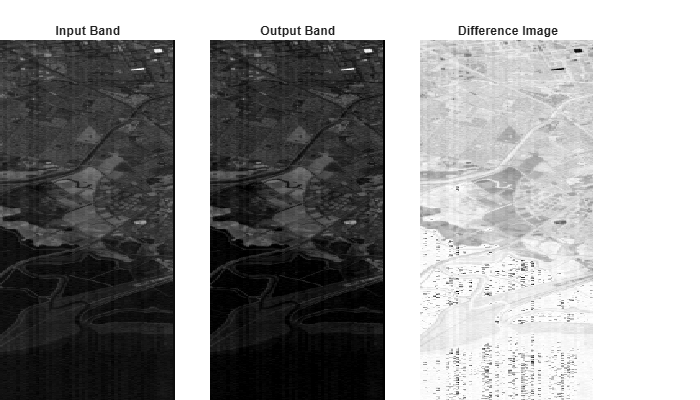
Inspect the results by selecting the same band image from both the uncalibrated digital number hypercube and the calibrated hypercube. For visualization purposes, rescale the values of the two band images to the range [0, 1]. Calculate the absolute value of the difference between the rescaled band images.
datacube = gather(hcube);
inputBand = rescale(datacube(:,:,159));
datacube_empirical = gather(hcube_empirical);
outputBand = rescale(datacube_empirical(:,:,159));
diffBand = abs(inputBand-outputBand);
Display the original spectral band image, the empirically corrected spectral band image, and the absolute value difference between the band images, to visualize the changes.
figure(Position=[0 0 700 400])
subplot(Position=[0 0 0.25 0.9])
imagesc(inputBand)
title("Input Band")
axis off
subplot(Position=[0.3 0 0.25 0.9])
imagesc(outputBand)
axis off
title("Output Band")
subplot(Position=[0.6 0 0.25 0.9])
imagesc(diffBand)
axis off
title("Difference Image")
colormap gray
Input Arguments
Output Arguments
Algorithms
The empiricalLine function performs linear regression for each band to
equate the digital number (DN), or TOA radiance or TOA reflectance, with the surface
reflectance. Solving the linear regression equation provides gain and offset values for each
band. This equation shows how the empirical line factors gain and offset values are calculated:
The gain (m) and the offset values (offset) are the unknown parameters in the empirical line equation. ρλ is the known surface reflectance value of a reference material in the input hyperspectral data (known as the field reference spectra). rλ is the measured value for the reference material in the input hyperspectral data (known as the image spectral data). The measured value can be a digital number, TOA radiance, or TOA reflectance.
The field reference spectra is an a priori measurement which can also be read from the spectral libraries. The empirical line approach solves the linear equation to find the gain and the offset values. The surface reflectance values for all the other pixels in the input hyperspectral data is calculated using the estimated gain and the offset values.
The empiricalLine function automatically resamples the input field
spectra to match the selected data wavelengths in hcube.
To solve the linear regression equation, at least two field spectrum values must be known
for each band. If the empiricalLine function is provided with only one field
spectrum value for each band, the offset value is set as zero. If there is no field spectrum
value available for any of the bands, then this function throws an error.
References
[1] Roberts, D. A., Y. Yamaguchi, and R. J. P. Lyon. "Comparison of Various Techniques for Calibration of AIS Data." In Proceedings of the Second Airborne Imaging Spectrometer Data Analysis Workshop, ed. Gregg Vane and Alexander F. H. Goetz, 21–30. Pasadena: Jet Propulsion Laboratory, 1986.
[2] Kruse, F. A., K. S. Kierein-Young, and J.W. Boardman. "Mineral Mapping at Cuprite, Nevada with a 63-Channel Imaging Spectrometer," Photogrammetric Engineering and Remote Sensing 56, no. 1 (January 1990): 83–92.
Version History
Introduced in R2020b
See Also
hypercube | iarr | flatField | logResiduals | subtractDarkPixel | reduceSmile | sharc