Adjust Image Contrast Using Histogram Equalization
This example shows how to adjust the contrast of a grayscale image using histogram equalization.
Histogram equalization involves transforming the intensity values so that the histogram of the output image approximately matches a specified histogram. By default, the histogram equalization function, histeq, tries to match a flat histogram with 64 bins such that the output image has pixel values evenly distributed throughout the range. You can also specify a different target histogram to match a custom contrast.
Original Image Histogram
Read a grayscale image into the workspace.
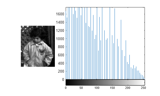
I = imread("pout.tif");Display the image and its histogram. The original image has low contrast, with most pixel values in the middle of the intensity range.
figure
subplot(1,3,1)
imshow(I)
subplot(1,3,2:3)
imhist(I)
Adjust Contrast Using Default Equalization
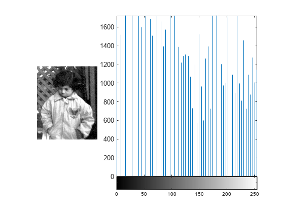
Adjust the contrast using histogram equalization. Use the default behavior of the histogram equalization function, histeq. The default target histogram is a flat histogram with 64 bins.
J = histeq(I);
Display the contrast-adjusted image and its new histogram.
figure
subplot(1,3,1)
imshow(J)
subplot(1,3,2:3)
imhist(J)
Adjust Contrast, Specifying Number of Bins
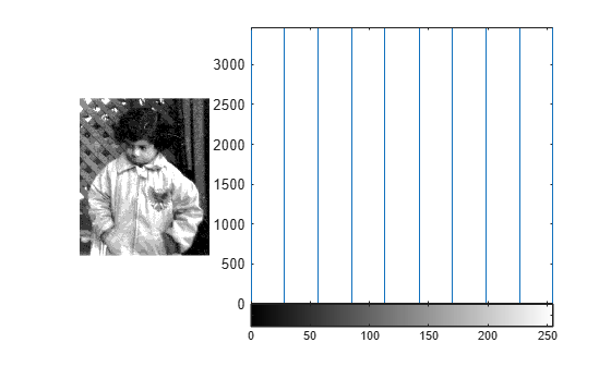
Adjust the contrast, specifying a different number of bins. With a small number of bins, there are noticeably fewer gray levels in the contrast-adjusted image.
nbins = 10;
K = histeq(I,nbins);
10;
K = histeq(I,nbins);Display the contrast-adjusted image and its new histogram.
figure
subplot(1,3,1)
imshow(K)
subplot(1,3,2:3)
imhist(K)
Adjust Contrast, Specifying Target Distribution
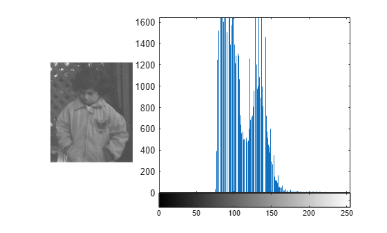
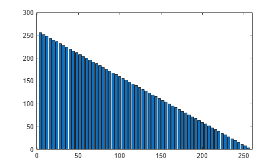
Adjust the contrast, specifying a nonflat target distribution. This example demonstrates a linearly decreasing target histogram, which emphasizes small pixel values and causes shadows to appear darker. Display the target histogram.
target = 256:-4:4;
figure
bar(4:4:256,target)
Adjust the histogram of the image to approximately match the target histogram.
L = histeq(I,target);
Display the contrast-adjusted image and its new histogram.
figure
subplot(1,3,1)
imshow(L)
subplot(1,3,2:3)
imhist(L)