Enhance Color Separation Using Decorrelation Stretching
Decorrelation stretching enhances the color separation of an image with significant
band-to-band correlation. The exaggerated colors improve visual interpretation and make
feature discrimination easier. You apply decorrelation stretching with the decorrstretch function. See Linear Contrast Stretching on how to add an optional linear contrast stretch
to the decorrelation stretch.
The number of color bands, NBANDS, in the image is usually three. But you can apply decorrelation stretching regardless of the number of color bands.
The original color values of the image are mapped to a new set of color values with a wider range. The color intensities of each pixel are transformed into the color eigenspace of the NBANDS-by-NBANDS covariance or correlation matrix, stretched to equalize the band variances, then transformed back to the original color bands.
To define the band-wise statistics, you can use the entire original image or, with the
subset option, any selected subset of it.
Simple Decorrelation Stretching
This example shows how to perform decorrelation stretching to three color bands of an image. A color band scatterplot of the images shows how the bands are decorrelated and equalized.
Perform Decorrelation Stretch
Read an image from the library of images available in the imdata folder. This example uses a LANDSAT image of the Little Colorado River. The image has seven bands, but just read in the three visible colors.
A = multibandread("littlecoriver.lan",[512 512 7], ...
  "uint8=>uint8",128,"bil","ieee-le", ...
  {"Band","Direct",[3 2 1]});
Perform the decorrelation stretch.
B = decorrstretch(A);
Display the original image and the processed image. Compare the two images. The original has a strong violet (red-bluish) tint, while the transformed image has a somewhat expanded color range.
imshow(A)
title("Little Colorado River Image")
imshow(B)
title("Little Colorado River Image After Decorrelation Stretch")
Create a Color Band Scatterplot
First separate the three color channels of the original image.
[rA,gA,bA] = imsplit(A);
Separate the three color channels of the image after decorrelation stretching.
[rB,gB,bB] = imsplit(B);
Display the color scatterplot of the original image. Then display the color scatterplot of the image after decorrelation stretching.
figure
plot3(rA(:),gA(:),bA(:),".")
grid on
xlabel("Red (Band 3)")
ylabel("Green (Band 2)")
zlabel("Blue (Band 1)")
title("Color Scatterplot Before Decorrelation Stretch")
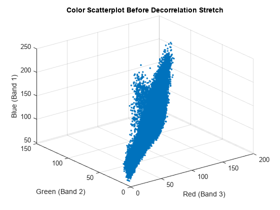
figure
plot3(rB(:),gB(:),bB(:),".")
grid on
xlabel("Red (Band 3)")
ylabel("Green (Band 2)")
zlabel("Blue (Band 1)")
title("Color Scatterplot After Decorrelation Stretch")

Linear Contrast Stretching
Adding linear contrast stretch enhances the resulting image by further expanding the
color range. The following example uses the Tol option to saturate equal
fractions of the image at high and low intensities. Without the Tol
option, decorrstretch applies no linear contrast stretch.
See the stretchlim function reference page for more
about calculating saturation limits.
Note
You can apply a linear contrast stretch as a separate operation after performing a
decorrelation stretch, using stretchlim and imadjust. This alternative, however, often gives inferior results for
uint8 and uint16 images, because the pixel values
must be clamped to [0 255] (or [0 65535]). The Tol option in
decorrstretch circumvents this limitation.
Decorrelation Stretch with Linear Contrast Stretch
Read the three visible color channels of the LANDSAT image of the Little Colorado River.
A = multibandread('littlecoriver.lan', [512, 512, 7], ...
  'uint8=>uint8', 128, 'bil', 'ieee-le', ...
  {'Band','Direct',[3 2 1]});
Apply decorrelation stretching, specifying the linear contrast stretch. Setting the value 'Tol' to 0.01 maps the transformed color range within each band to a normalized interval between 0.01 and 0.99, saturating 2%.
C = decorrstretch(A,'Tol',0.01);
imshow(C)
title(['Little Colorado River After Decorrelation Stretch and ',...
  'Linear Contrast Stretch'])

See Also
decorrstretch | imadjust | stretchlim | imhist | multibandread | plot3