Estimate States of Nonlinear System with Multiple, Multirate Sensors
This example shows how to perform nonlinear state estimation in Simulink® for a system with multiple sensors operating at different sample rates. The Extended Kalman Filter block in System Identification Toolbox™ is used to estimate the position and velocity of an object using GPS and radar measurements.
Introduction
The toolbox has three Simulink blocks for nonlinear state estimation:
Extended Kalman Filter: Implements the first-order discrete-time extended Kalman filter algorithm.
Unscented Kalman Filter: Implements the discrete-time unscented Kalman filter algorithm.
Particle Filter: Implements a discrete-time particle filter algorithm.
These blocks support state estimation using multiple sensors operating at different sample rates. A typical workflow for using these blocks is as follows:
Model your plant and sensor behavior using MATLAB® or Simulink functions.
Configure the parameters of the block.
Simulate the filter and analyze results to gain confidence in filter performance.
Deploy the filter on your hardware. You can generate code for these filters using Simulink Coder™ software.
This example uses the Extended Kalman Filter block to demonstrate the first two steps of this workflow. The last two steps are briefly discussed in the Next Steps section. The goal in this example is to estimate the states of an object using noisy measurements provided by a radar and a GPS sensor. The states of the object are its position and velocity, which are denoted as xTrue in the Simulink model.
If you are interested in the Particle Filter block, see the example "Parameter and State Estimation in Simulink Using Particle Filter Block".
open_system('multirateEKFExample');Plant Modeling
The extended Kalman filter (EKF) algorithm requires a state transition function that describes the evolution of states from one time step to the next. The block supports the following two function forms:
Additive process noise:
Nonadditive process noise:
Here f(..) is the state transition function, x is the state, and w is the process noise. u is optional, and represents additional inputs to f, for instance system inputs or parameters. Additive noise means that the next state and process noise are related linearly. If the relationship is nonlinear, use the nonadditive form.
The function f(...) can be a MATLAB Function that complies with the restrictions of MATLAB Coder™, or a Simulink Function block. After you create f(...), you specify the function name and whether the process noise is additive or nonadditive in the Extended Kalman Filter block.
In this example, you are tracking the north and east positions and velocities of an object on a 2-dimensional plane. The estimated quantities are:
.
Here is the discrete-time index. The state transition equation used is of the nonadditive form , where is the state vector, and is the process noise. The filter assumes that is a zero-mean, independent random variable with known variance . The A and G matrices are:
where is the sample time. The third row of A and G model the east velocity as a random walk: . In reality, position is a continuous-time variable and is the integral of velocity over time . The first row of A and G represent a discrete approximation to this kinematic relationship: . The second and fourth rows of A and G represent the same relationship between the north velocity and position. This state transition model is linear, but the radar measurement model is nonlinear. This nonlinearity necessitates the use of a nonlinear state estimator such as the extended Kalman filter.
In this example you implement the state transition function using a Simulink Function block. To do so,
Add a Simulink Function block to your model from the
Simulink/User-Defined FunctionslibraryClick on the name shown on the Simulink Function block. Edit the function name, and add or remove input and output arguments, as necessary. In this example the name for the state transition function is
stateTransitionFcn. It has one output argument (xNext) and two input arguments (x, w).

Though it is not required in this example, you can use any signals from the rest of your Simulink model in the Simulink Function. To do so, add
Inportblocks from theSimulink/Sourceslibrary. Note that these are different than theArgInandArgOutblocks that are set through the signature of your function (xNext = stateTransitionFcn(x, w)).In the Simulink Function block, construct your function utilizing Simulink blocks.
Set the dimensions for the input and output arguments x, w, and xNext in the Signal Attributes tab of the
ArgInandArgOutblocks. The data type and port dimensions must be consistent with the information you provide in the Extended Kalman Filter block.

Analytical Jacobian of the state transition function is also implemented in this example. Specifying the Jacobian is optional. However, this reduces the computational burden, and in most cases increases the state estimation accuracy. Implement the Jacobian function as a Simulink function because the state transition function is a Simulink function.
open_system('multirateEKFExample/Simulink Function - State Transition Jacobian');Sensor Modeling - Radar
The Extended Kalman Filter block also needs a measurement function that describes how the states are related to measurements. The following two function forms are supported:
Additive measurement noise:
Nonadditive measurement noise:
Here h(..) is the measurement function, and v is the measurement noise. u is optional, and represents additional inputs to h, for instance system inputs or parameters. These inputs can differ from the inputs in the state transition function.
In this example a radar located at the origin measures the range and angle of the object at 20 Hz. Assume that both of the measurements have about 5% noise. This can be modeled by the following measurement equation:
.
Here and are the measurement noise terms, each with variance 0.05^2. That is, most of the measurements have errors less than 5%. The measurement noise is nonadditive because and are not simply added to the measurements, but instead they depend on the states x. In this example, the radar measurement equation is implemented using a Simulink Function block.
open_system('multirateEKFExample/Simulink Function - Radar Measurements');Sensor Modeling - GPS
A GPS measures the east and north positions of the object at 1 Hz. Hence, the measurement equation for the GPS sensor is:
Here and are measurement noise terms with the covariance matrix [10^2 0; 0 10^2]. That is, the measurements are accurate up to approximately 10 meters, and the errors are uncorrelated. The measurement noise is additive because the noise terms affect the measurements linearly.
Create this function, and save it in a file named gpsMeasurementFcn.m. When the measurement noise is additive, you must not specify the noise terms in the function. You provide this function name and measurement noise covariance in the Extended Kalman Filter block.
type gpsMeasurementFcnfunction y = gpsMeasurementFcn(x) % gpsMeasurementFcn GPS measurement function for state estimation % % Assume the states x are: % [EastPosition; NorthPosition; EastVelocity; NorthVelocity] %#codegen % The %#codegen tag above is needed is you would like to use MATLAB Coder to % generate C or C++ code for your filter y = x([1 2]); % Position states are measured end
Filter Construction
Configure the Extended Kalman Filter block to perform the estimation. You specify the state transition and measurement function names, initial state and state error covariance, and process and measurement noise characteristics.
In the System Model tab of the block dialog box, specify the following parameters:
State Transition
Specify the state transition function,
stateTransitionFcn, in Function. Since you have the Jacobian of this function, select Jacobian, and specify the Jacobian function,stateTransitionJacobianFcn.Select
Nonadditivein the Process Noise drop-down list because you explicitly stated how the process noise impacts the states in your function.Specify the process noise covariance as [0.2 0; 0 0.2]. As explained in the Plant Modeling section of this example, process noise terms define the random walk of the velocities in each direction. The diagonal terms approximately capture how much the velocities can change over one sample time of the state transition function. The off-diagonal terms are set to zero, which is a naive assumption that velocity variations in the north and east directions are uncorrelated.
Initialization
Specify your best initial state estimate in Initial state. In this example, specify [100; 100; 0; 0].
Specify your confidence in your state estimate guess in Initial covariance. In this example, specify 10. The software interprets this value as the true state values are likely to be within of your initial estimate. You can specify a separate value for each state by setting
Initial covarianceas a vector. You can specify cross-correlations in this uncertainty by specifying it as a matrix.
Since there are two sensors, click Add Measurement to specify a second measurement function.
Measurement 1
Specify the name of your measurement function,
radarMeasurementFcn, in Function.Select
Nonadditivein the Measurement Noise drop-down list because you explicitly stated how the process noise impacts the measurements in your function.Specify the measurement noise covariance as [0.05^2 0; 0 0.05^2] per the discussion in the Sensor Modeling - Radar section.
Measurement 2
Specify the name of your measurement function,
gpsMeasurementFcn, in Function.This sensor model has additive noise. Therefore, specify the GPS measurement noise as
Additivein the Measurement Noise drop-down list.Specify the measurement noise covariance as [100 0; 0 100].

In the Multirate tab, since the two sensors are operating at different sample rates, perform the following configuration:
Select
Enable multirate operation.Specify the state transition sample time. The state transition sample time must be the smallest, and all measurement sample times must be an integer multiple of the state transition sample time. Specify State Transition sample time as 0.05, the sample time of the fastest measurement. Though not required in this example, it is possible to have a smaller sample time for state transition than all measurements. This means there will be some sample times without any measurements. For these sample times the filter generates state predictions using the state transition function.
Specify the Measurement 1 sample time (Radar) as 0.05 seconds and Measurement 2 (GPS) as 1 seconds.

Simulation and Results
Test the performance of the Extended Kalman filter by simulating a scenario where the object travels in a square pattern with the following maneuvers:
At t = 0, the object starts at
It heads north at until t = 20 seconds.
It heads east at between t = 20 and t = 45 seconds.
It heads south at between t = 45 and t = 85 seconds.
It heads west at between t = 85 and t = 185 seconds.
Generate the true state values corresponding to this motion:
Ts = 0.05; % [s] Sample rate for the true states
[t, xTrue] = generateTrueStates(Ts); % Generate position and velocity profile over 0-185 seconds
Simulate the model. For instance, look at the actual and estimated velocities in the east direction:
sim('multirateEKFExample');
open_system('multirateEKFExample/Scope - East Velocity');
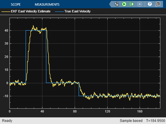
The plot shows the true velocity in the east direction, and its extended Kalman filter estimates. The filter successfully tracks the changes in velocity. The multirate nature of the filter is most apparent in the time range t = 20 to 30 seconds. The filter makes large corrections every second (GPS sample rate), while the corrections due to radar measurements are visible every 0.05 seconds.
Next Steps
Validate the state estimation: The validation of unscented and extended Kalman filter performance is typically done using extensive Monte Carlo simulations. For more information, see Validate Online State Estimation in Simulink.
Generate code: The Unscented and Extended Kalman Filter blocks support C and C++ code generation using Simulink Coder software. The functions you provide to these blocks must comply with the restrictions of MATLAB Coder software (if you are using MATLAB functions to model your system) and Simulink Coder software (if you are using Simulink Function blocks to model your system).
Summary
This example has shown how to use the Extended Kalman Filter block in System Identification Toolbox. You estimated position and velocity of an object from two different sensors operating at different sampling rates.
close_system('multirateEKFExample', 0);See Also
Extended Kalman Filter | Unscented Kalman Filter | Particle Filter