Dynamic System Learner

R2026b

Train models for time series prediction

Since R2026b

Description

Use the Dynamic System Learner app to train models for time series prediction.

Using this app, you can:

• Import and visualize time series data. You can also specify data preprocessing options such as normalization and splitting the data into training and validation sets.

• Train models for time series prediction. You can select and adapt predefined models.

• Monitor training metrics of trained candidate models.

• Use your trained model to predict values for the training and validation data sets.

• Track and compare the performance of trained models.

• Generate code to help you predict on new data.

• Export your model to Simulink^® layer blocks for integration of your model into a larger engineering system.

Available Models

• Autoregressive moving average with exogenous input (ARMAX) model.

• Nonlinear autoregressive with exogenous input (ARX) model.

• Long short-term memory (LSTM) networks. These networks require Deep Learning Toolbox™.

• Gated recurrent unit (GRU) networks. These networks require Deep Learning Toolbox.

• Multi-layer perceptron (MLP) networks. These networks require Deep Learning Toolbox.

• Convolutional neural networks (CNN). These networks require Deep Learning Toolbox.

• Custom deep neural networks suitable for one-step-ahead time series modeling. These networks require Deep Learning Toolbox.

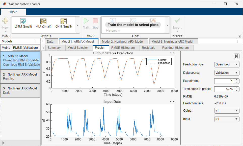
Open the Dynamic System Learner App

• MATLAB^® Toolstrip: On the Apps tab, under Control System Design and Analysis, click the app icon.

• MATLAB command prompt: Enter dynamicSystemLearner.

Examples

• Estimate ARMAX Model Using Dynamic System Learner App
• Estimate Nonlinear ARX Model Using Dynamic System Learner App
• Predict Battery State-Of-Charge Using Dynamic System Learner App

Parameters

New — Import data from workspace

button

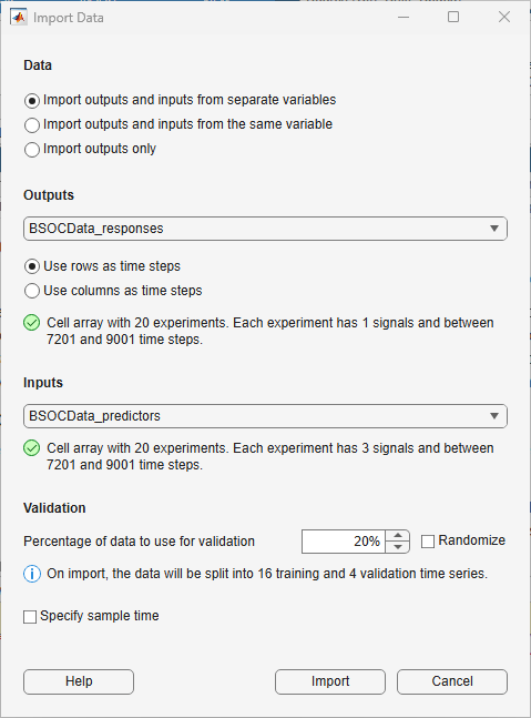
When you click New > Numeric or timetable , the app opens the Import Data dialog box. Use the dialog box to specify these options: Data, Outputs, Data Set Variable, Time step dimension, Inputs, Validation, Randomize, and Specify sample time.

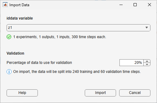
When you click New > iddata, the app opens a different Import Data dialog box. In the dialog box, under iddata variable, select an iddata object from the workspace. Also specify the Validation option.

Data — Location of outputs and inputs

radio button

Specify the data type and location as one of these options:

• Import outputs and inputs from separate variables

• Import outputs and inputs from the same variable

• Import outputs only

If you import the outputs and inputs from the same variable, then the app displays a table where you can select which signals are outputs and which signals are inputs. For more information, see Inputs.

Outputs — Data to use for training

numeric array | cell array | table | timetable object

In the Outputs list, select the variable to use to train your model to predict, specified as a numeric array, cell array, table, or timetable object. For timetable data, the data must be sampled at regular intervals. For other input types, the app assumes that the data is sampled at regular intervals.

Dependencies

This option is only available if Data is Import outputs and inputs from separate variables or Import outputs only.

Data Set Variable — Data to use for training

numeric array | cell array | table | timetable object

In the Data Set Variable list, select the variable to use to train your model, specified as a numeric array, cell array, table, or timetable object. For timetable data, the data must be sampled at regular intervals. For other input types, the app assumes that the data is sampled at regular intervals.

Dependencies

This option is only available if Data is Import outputs and inputs from the same variable.

Time step dimension — Dimension of time steps

Use rows as time steps (default) | Use columns as time steps

Specify the format for the time series data. The app accepts time series data in either "TC" (time, channel) or "CT" (channel, time) format.

• For "TC" data, select Use rows as time steps.

• For "CT" data, select Use columns as time steps.

Tips

For each option, the app displays information about your data, such as the number of time series, number of signals, and length of the time steps. Use this information to check that you have specified the correct time dimension.

Inputs — Input data

numeric array | cell array | table | timetable object

In the Inputs list, specify additional variables that are related, but are not part of, the time series you want to model.

• If Data is Import outputs and inputs from separate variables, then select the inputs variable. The input data must be specified as a numeric array, cell array, table, or timetable object that is compatible with the output data. The app assumes that the input data is sampled at regular intervals.

• If Data is Import outputs and inputs from the same variable, then use the table to select which signals are outputs and which signals are inputs.

Dependencies

This option is only available if Data is Import outputs and inputs from separate variables or Import outputs and inputs from the same variable.

If you import a separate input variable, then the data type of the output variable and the inputs must match. For example, if you specify the outputs as a table, then the inputs must also be a table.

Validation — Percentage of data to use for validation

20% (default) | nonnegative scalar less than 100%

In the Validation section, specify the percentage of data to use for validation.

The validation split depends on how many time series you have. Suppose that you specify Validation as a value val:

• If you have a single time series, then the validation data is the last val% of the time steps. For example, if you have a single time series with 100 time steps and a validation split of 30%, then the app uses the first 70 time steps for training and the last 30 time steps for validation.

• If you have multiple time series, then the validation data is val% of the time series. For example, if you have 100 time series and a validation split of 30%, then the app uses 70 time series for training and 30 time series for validation.

Tips

Monitoring the performance of the model on the validation data is important for detecting overfitting. For more information, see Training Diagnostics.

Randomize — Flag to randomize validation data split

'off' (default) | 'on'

Select the Randomize check box to randomly assign the specified proportion of experiments to the validation data set.

Tips

Randomizing the validation data can improve the accuracy of networks trained on data stored in a nonrandom order.

Dependencies

This option is only available if your data contains multiple experiments.

Specify sample time — Specify fixed sample time

'off' (default) | 'on'

Select the Specify sample time check box to specify the sample time and the units of the time steps in your data. When you select this option, the app displays these additional options:

• Sample time — Size of each time step, specified as a positive scalar.

• Units — Units of the time step, specified as seconds, minutes, hours, or days.

If you specify the time step size and units, the app labels the x-axis of the plots with the corresponding time values. The time step information is available in the experiment preview, predict plot, and residuals plot. This option affects the plots only.

Note

If you do not specify the time step, the app labels plot axes using time step indices.

Data — Preview input data

tab

After you import data, the app displays a summary of the data in the Data tab. You can also preview individual experiments.

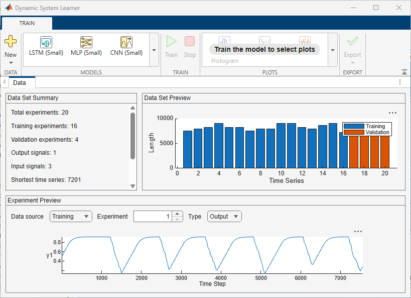
Dependencies

The plots you see in the Data tab depend on whether your data contains a single experiment or multiple experiments.

Model — Time series model

LSTM (Small) | LSTM (Large) | MLP (Small) | CNN (Small) | From Workspace | Blank Network | ARMA Model | ...

In the model gallery, select a model to train for time series modeling.

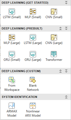
The model gallery contains template models that you can use or adapt for your task. The app includes the ARMAX and nonlinear ARX models. When you choose the ARMAX model, the app displays the equation of the model structure along with the structure configuration options. When you choose the nonlinear ARX model, the app displays a diagram of the regressors and the output function along with the structure configuration options. If you have Deep Learning Toolbox, then the app also includes several built-in deep learning models in small and large variants. You can customize these models by changing their parameters or by using the interactive editor. If you require more customization, then you can import a dlnetwork object from the workspace or create a network from scratch using the network editor. For more information, see Customize Network. When you choose a deep learning model, the app displays a plot of the network architecture.

For deep learning models, in the Model tab, you can specify Data Preprocessing, Model Hyperparameters, and Training Options. To make custom edits to your model, see Customize Network. For the ARMAX and nonlinear ARX models, in the Summary tab under Model, you can specify Model Structure and Training Options.

You can track, manage, and compare models in the Models pane. Before training, the model is in Draft status and you can edit its properties. After training, the Models pane displays the metrics for the model, reported over the training and validation data. For more information, see Training Results. You can duplicate your model options into a new draft by clicking the Duplicate button . You can also delete a model by clicking the Delete button .

Predefined Models

Most of the predefined deep learning models have a small and a large version. The small versions have fewer learnable parameters and layers and do not include dropout layers. The large versions have more learnable parameters and layers and include dropout layers. The small models are faster to train, whereas the large models can learn more complex features.

The app supports small and large versions of these models, which require Deep Learning Toolbox:

• LSTM — Long short-term memory network, a type of recurrent network that can capture long-term dependencies in sequence data.

• MLP — Multi-layer perceptron, a type of feedforward network where each layer is fully connected to the next.

• GRU — Gated recurrent unit, a type of recurrent network that can capture long-term dependencies in sequence data. GRU networks are simplified and potentially more computationally efficient versions of LSTM networks.

• CNN — Convolutional neural network, a type of feedforward network that learns features by applying sliding convolutional filters to 1-D input.

The app also supports the ARMAX model and the nonlinear ARX model. For more information on training ARMAX and nonlinear ARX models, see Estimate ARMAX Model Using Dynamic System Learner App and Estimate Nonlinear ARX Model Using Dynamic System Learner App.

Custom Deep Learning Networks

You can use the app to create and train custom deep learning models. Using the app, you can:

• Adapt any of the predefined models. To adapt a model, click Customize Network.

• Import a dlnetwork (Deep Learning Toolbox) object suitable for time series modeling tasks. To import a dlnetwork object, click From Workspace.

• Open a blank canvas for network creation. To open a canvas, click Blank Network .

Custom models must be compatible with your data. For a list of requirements, see Customize Network.

Model Options

Data Preprocessing — Data preprocessing options

panel section

Use the Data Preprocessing options to control how the network processes the data. These options are available only for deep learning models.

• Use past values of responses as inputs (default 'off') — Select this option to use an autoregressive model. Consider using an autoregressive model when past values of the response time series influence future predictions. Autoregressive models are often slower than nonautoregressive models at predicting on new data.

• Normalize experiments (default 'on') — Select this option to normalize the training and validation data. When you select this option, the network normalizes the input data at the sequence input layer and denormalizes it at the inverse normalization layer. By default, the app normalizes the data, X, using z-score normalization:

  $$z=\frac{X-\mu }{\sigma }$$

  where μ is the mean and σ is the standard deviation of the training data across each channel.

  When training neural networks, normalization helps stabilize and speeds up network training using gradient descent. If your data is poorly scaled, then during training, the loss can become NaN and the network parameters can diverge.

• Sort experiments by length (default 'on') — Select this option to enable sorting the time series by length. By default, the app sets the SequenceLength training option to longest. This setting causes the software to pad the sequences so that all the sequences in a mini-batch have the same length as the longest sequence in the mini-batch. Sorting experiments by length reduces the amount of padding or discarded data when padding or truncating sequences. If you do not sort experiments length, then you might see different results. For more information, see SequenceLength (Deep Learning Toolbox).

  This option is only available if your time series data contains multiple experiments.

• Split time series into windows — Split the time series training data into windows (chunks). Splitting the training data into shorter windows can improve training time and accuracy. This option is only available if you have a single, long experiment. If you enable this option, then the app might not use all of the data for training. The amount of discarded data depends on the length of the time series, the window length, and the window stride. For example, for a time series with 1,010 time steps, a window length of 200, and a stride of 200, the app will split the time series into five windows and discards the final 10 time steps.

  Window options

  • Window length — Number of time steps to include in each window of data. The window length needs to be long enough to capture relevant patterns but not too long to dilute them.

  • Window stride — Number of time steps between each window. When the stride is less than the window length, then windows will overlap. Smaller strides give more overlap (more data, slower training); larger strides reduce overlap (faster, but less data).

Model Hyperparameters — Model architecture options

panel section

Use the Model Hyperparameters options to control the network architecture. These options are only available for the predefined deep neural networks. If you customize the network using the Customize Network button, then these options are not available.

• Network depth (blocks) — This option specifies the number of repeating blocks, where the blocks depend on which network you select. For example, for an LSTM network with a dropout probability greater than 0, the repeating blocks are an LSTM layer followed by a dropout layer.

• Hidden units — This option specifies the number of hidden units (also known as the hidden size) in each of the layers with learnable parameters. The number of hidden units corresponds to the amount of information that the layer remembers between time steps. If the number of hidden units is too large, then the layer can overfit to the training data.

  This option is supported for LSTM, GRU, and MLP networks only.

• Filter size — This option specifies the width of the filters in the 1-D convolutional layers.

  This option is supported for CNNs only.

• Filters — This option specifies the number of filters in the 1-D convolutional layers. This number corresponds to the number of neurons in the layer that connect to the same region in the input. This parameter determines the number of channels (feature maps) in the layer output.

  This option is supported for CNNs only.

• Dropout probability — This option specifies the dropout probability for each of the dropout layers in the network.

  • If the dropout probability is 0, then the network does not contain any dropout layers.

  • If the dropout probability is greater than 0, then the network contains dropout layers with the specified dropout probability. The number of dropout layers depends on the network depth.

  For more information, see dropoutLayer (Deep Learning Toolbox).

Customize Network — Customize neural network

button

This button is only available for deep learning models.

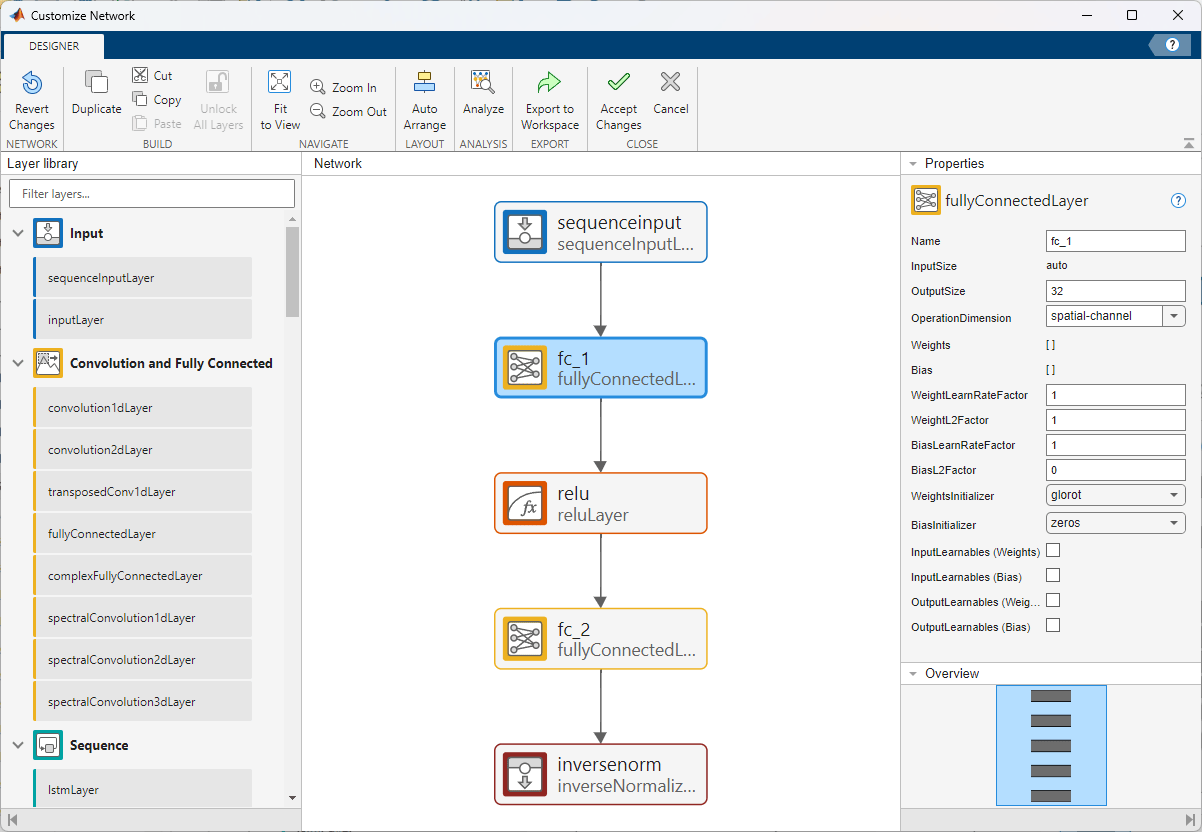
After you select a predefined deep learning network, click Customize Network to open a window for network editing. The app opens the network editing window with input and output layers suitable for your task. The network editor is a simplified version of the Deep Network Designer (Deep Learning Toolbox) app that is tailored for constructing and configuring networks for time series modeling tasks. For more information about building deep neural networks, see Build Networks with Deep Network Designer (Deep Learning Toolbox).

You can use the Customize Network window to add or delete layers and to change network parameters. To check the edited network for issues, click Analyze. When you are happy with your changes, click Accept Changes to accept the network changes.

Dependencies

If you edit a network or create one from scratch, then the network must be suitable for sequence-to-sequence regression tasks. If you select Use past values of responses as inputs, then the network must also be suitable for tasks where you also use the responses as inputs with a time lag of 1.

The network must also be compatible with the imported data in these ways.

• The network must have a single input layer and a single output layer.

• The input size must match the input size of the imported data. If you select Use past values of responses as inputs, then the input size must be Number of Response Channels + Number of Predictor Channels. If you do not select Use past values of responses as inputs, then the input size must be Number of Predictor Channels.

• The output size must match the output size of the imported data, where the output size of the imported data is Number of Response Channels.

• The input and output format must match the input and output format of the data.

• If the input layer is a sequenceInputLayer and you select Use past values of responses as inputs, then the MinLength property must be less than the minimum sequence length in the imported data. If the input layer is a sequenceInputLayer and you do not select Use past values of responses as inputs, then the MinLength property must be less than or equal to the minimum sequence length in the imported data.

• If the input layer is an inputLayer, then the time dimension of the InputSize property must be less than or equal to the minimum sequence length in the imported data.

• The size of the time dimension on the input layer must match that of the output layer.

• If the input layer has a SplitComplexInput property, then this property must be set to false.

Model Structure — Model structure options

panel section

Use the Model Structure options to specify the structure of the model. These options are available only for the ARMAX model.

• Configuration choice — Select Configuration choice as either Specify maximum lag only or Specify orders. Each choice gives you a different set of options to configure.

• Include integration — This option specifies to include the integrator in the model structure.

• Input-Output Delay — This option specifies the input-output delay, also known as the transport delay. It appears only when you import both outputs and inputs.

For more information on the model structure options, see Model Structure Configuration.

These options are available only for the nonlinear ARX model.

• Regressor Specification — To specify regressors, select either Create Regressors or Extend Linear Model. Each choice gives you a different set of options to configure.

• Output Functions — Select the output function that maps the regressors of the nonlinear ARX model into the model output as Linear, Sigmoid Network, Wavelet Network, or Custom Network, and configure the options that appear.

For more information on the nonlinear ARX model structure options, see Model Structure Configuration.

Training Options — Training options

panel section

Use the Training Options options to control how the app trains the model. These options are only available for deep learning models.

• InitialLearnRate — This option specifies the initial learning rate to use for training. If the learning rate is too low, then training can take a long time. If the learning rate is too high, then training might reach a suboptimal result or diverge.

  When the Solver option is sgdm, the default value is 0.01. When Solver is rmsprop or adam, the default value is 0.001. To set the Solver option, click Show advanced options and then click Solver.

  For more information, see InitialLearnRate (Deep Learning Toolbox).

• MiniBatchSize — This option specifies the mini-batch size to use for training. A mini-batch is a subset of the training set that is used to evaluate the gradient of the loss function and update the weights. If the mini-batch size does not evenly divide the number of training samples, then the software discards the training data that does not fit into the last complete mini-batch of each epoch. If the mini-batch size is smaller than the number of training samples, then the software does not discard any data.

  For more information, see MiniBatchSize (Deep Learning Toolbox).

• MaxEpochs — This option specifies the maximum number of epochs (full passes of the data) to use for training.

  For more information, see MaxEpochs (Deep Learning Toolbox).

• Show advanced options — Select this option to specify additional training options. For more information about these training options, see trainingOptions (Deep Learning Toolbox).

These options are only available for the ARMAX model.

• Focus on simulation (long time-horizon prediction) fidelity — Select this option to minimize the simulation error between measured and simulated outputs during estimation. As a result, the estimation focuses on making a good fit for simulation of model response with the current inputs. This option is available only when you import both outputs and inputs.

• Enforce model stability — Select this option to enforce stability of the estimated model.

• Maximum iterations — This option specifies the maximum number of iterations during loss-function minimization, as a nonnegative integer. The iterations stop when MaxIterations is reached or another stopping criterion is satisfied, such as Tolerance. Specifying MaxIterations as 0 returns the result of the start-up procedure.

• Tolerance — This option specifies the minimum percentage difference between the current value of the loss function and its expected improvement after the next iteration, as a positive scalar. When the percentage of expected improvement is less than Tolerance, the iterations stop. The estimate of the expected loss-function improvement at the next iteration is based on the Gauss-Newton vector computed for the current parameter value.

• Robustify training against data outliers — Select this option to strengthen training against data outliers.

• Use parallel computation — Select this option to enable parallel computing for model training. You use parallel computing to simultaneously train multiple candidate models based on the model structure you specify.

These options are only available for nonlinear ARX models.

General

• Focus on simulation (long time-horizon prediction) fidelity — Select this option to minimize the simulation error between measured and simulated outputs during estimation. The estimation focuses on making a good fit for simulation of model response with the current inputs. This option is available only when you import both outputs and inputs.

• Window size — This option specifies the number of samples in each frame or batch when segmenting data for model training, as a positive integer.

• Automatically select overlap — Select this option to automatically select the size of the overlap to be equal to the maximum delay across all model regressors.

• Overlap — This option specifies the number of samples in the overlap between successive frames when segmenting data for model training, as an integer. A negative integer indicates that certain data samples are skipped when creating the data frames. You can specify this option only if you do not select Automatically select overlap.

• Use parallel computation — Select this option to enable parallel computing for model training. Use parallel computing to simultaneously train multiple candidate models based on the model structure you specify.

Search Options

• Search method — This option specifies the numerical search method to use for iterative parameter estimation as Auto, Gauss-Newton (gn), Adaptive Gauss-Newton (gna), Levenberg-Marquardt (lm), Gradient Descent (grad), Trust-region Reflective Newton (lsqnonlin), Pattern Search (patternsearch), or Constrained Nonlinear Optimization (fmincon). Each method has associated options that you can configure.

Normalization Options

• Normalize — Select this option to normalize estimation data using the method specified in Normalization Method.

• Normalization Method — This option specifies the method to use to normalize estimation data as Auto, Center, Z-Score, Norm, Scale, Range, or Median Interquartile Range. Some methods have an associated option that you can configure.

For more information on nonlinear ARX model training options, see Training Options Configuration.

Closed Loop Metric Evaluation Options — Options for closed loop metric evaluation

panel section

Use the Closed Loop Metric Evaluation Options to control how the app evaluates the metrics during closed loop evaluation. These options only apply to the metric evaluation after training. The results of the metric evaluation appear in the Training Results section. These options are only available for deep learning models.

• Use stateful prediction — Update the network state every iteration during closed loop prediction. Select this option if your model architecture supports statefulness (for example, LSTM or GRU) and each prediction depends on the previous one.

• Initial context length — Number of time steps of true values to use as the initial context of the first prediction during closed loop prediction.

• Sliding window length — Number of time steps to use as input at each subsequent prediction step during closed loop prediction. After the initial prediction, the model slides through the time series as it makes predictions. Choose a window length that captures enough information to make the prediction. A window length that is too short can cause the model to miss trends, and a window length that is too long can add noise or complexity to the predictions. If you have only output data, then you might need a longer window length in order to make accurate predictions.

Dependencies

These options only appear when you select Use past values of responses as inputs that is, when you use an autoregressive model.

The default sliding window length depends on the network. For most networks, using stateful prediction with a sliding window length value greater than 1 will produce poor results. By default, the app does not use stateful prediction if the sliding window length is greater than one.

Training Results — Training metrics

panel section

The Training Results appear in the Summary tab after you have trained the model. For deep learning models, the app reports the loss (RMSE) and MAE values over the entire training and validation data as a full pass through the network. If the value of Use past responses as inputs is true, then the app also displays the closed loop RMSE and MAE values. For more information, see Data Preprocessing. For the ARMAX and nonlinear ARX models, the app always displays both the closed-loop and open-loop values for RMSE and MAE.

Train — Train model

button

Click the Train button to train the model.

When training deep learning models, the app displays metrics for the MAE and model loss for both the training and validation data. For the training data, the app reports metrics for the current mini-batch. For the validation data, the app reports metrics over the full validation set by combining the results from all the validation mini-batches.

The app also displays information about the training and training diagnostics. When training the ARMAX and nonlinear ARX models, the app opens the Model Selector panel and displays the statement Trying various model structure and fitting algorithms... in the Training Information section.

Training Progress — Information about training

panel

This panel is only available for deep learning models.

When training deep learning models, the app displays the Training Information panel.

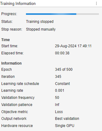
This panel contains this information:

• Progress — Progress bar indicating the training progress.

• Status — The training status. The status can be "Running" or "Training stopped".

• Stop reason — The reason why training stopped, such as that the max epochs was reached.

• Start time — The training start time.

• Elapsed time — The elapsed time during training.

• Epoch — The current epoch.

• Iteration — The current iteration.

• Learning rate schedule — The learning rate schedule used during training. This option is set using the advanced training option LearnRateSchedule.

• Learning rate — The current learning rate. This option depends on the InitialLearnRate, LearnRateSchedule, LearnRateDropPeriod, and LearnRateDropFactor training options.

• Validation frequency — Frequency of neural network validation. This option depends on the advanced training option ValidationFrequency.

• Validation patience — Patience of validation stopping. This option depends on the advanced training option ValidationPatience.

• Objective metric — Frequency of neural network validation. This option depends on the advanced training option ValidationFrequency.

• Output Network — Neural network to return when training completes. The app always returns the network with the lowest validation loss during training.

• Hardware resource — Hardware resource for training neural network. This option depends on the advanced training option ExecutionEnvironment.

For more information about the training options, see trainingOptions (Deep Learning Toolbox).

Training Diagnostics — Training diagnostic information

panel

During training, use the Training Diagnostics panel at the bottom of the app to see if your model has any issues. It is difficult to determine why a model has issues, but the app provides a list of general suggestions to help prevent issues when training a deep neural network. This information is available only for deep learning models. For more information, see Detect Issues When Training Model for Time Series Forecasting (Deep Learning Toolbox).

Tips

By default, the app returns the model with the best validation loss. So, even if your network is overfitting at the end of training, the app can return a model at the point of no overfitting. The network returned by the app is equivalent to stopping training when the validation loss stops decreasing.

Model Selector — Information about candidate models

panel

This panel is available only for the ARMAX and nonlinear ARX models.

After model training, the app produces anywhere between one to seven candidate models. A plot displaying this set of candidate models and their respective metric values appears on the Model Selector panel. At the top of the plot, in the Metric menu, you can choose the quality metric that you want the plot to display as RMSE, NRMSE, MAE, AIC, or BIC. If you select Metric as RMSE, NRMSE, or MAE, you can select Open-loop or Closed-loop at the top right of the plot to display the respective plots.

To the left of the plot, you can choose all the models that you want to display. You can choose to display the Training dataset, Validation dataset, or both.

The plot automatically highlights the model with the lowest NRMSE value on training data in the closed-loop metric setting. You can also see that the app selects this model in the Select model list and displays its information in the Model Details section. You can select a different model by clicking the model in the plot or selecting it in the Select model list.

After you select a model, click Apply to finalize the selection and complete the training process. After the app generates the candidate models, clicking Stop on the Train tab is equivalent to clicking Apply on the Model Selector panel.

For more information on model selection, see Train ARMAX Model or Train Nonlinear ARX Model.

Stop — Stop training

button

Click the Stop button to stop training the model. For deep learning models, you can still use the neural network even if you stop training early. The app returns the model with the best validation loss. For the ARMAX and nonlinear ARX models, if you click Stop before the app generates the candidate models, the app displays a training error. If you click Stop after the app generates the candidate models, the app finalizes the selected model and completes the training process.

Plots — Analyze network performance using plots

RMSE Histogram | Predict | Residuals | Residual Histogram

To analyze the performance of your model, you can generate these plots for either the training or validation data:

• RMSE Histogram — Click the RMSE Histogram button to plot a histogram of the RMSE values for each time series.

• Predict — Click the Predict button to use the trained model to predict values for a specified time series.

• Residuals — Click the Residuals button to plot the residuals for a specified time series. Residuals are the differences between the true response values and the values predicted by the model.

• Residual Histogram — Click the Residual Histogram button to plot a histogram of the residuals for a specified time series.

In the tab for each plot, you can specify options to configure that plot.

Prediction type — Type of prediction

Closed loop (default) | Open loop

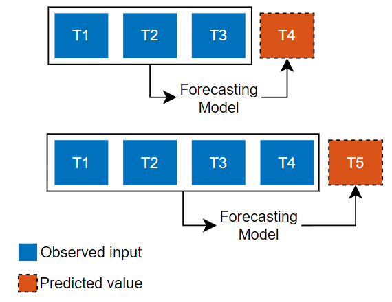
Use the Prediction type list to select the type of prediction.

Open Loop	Closed Loop
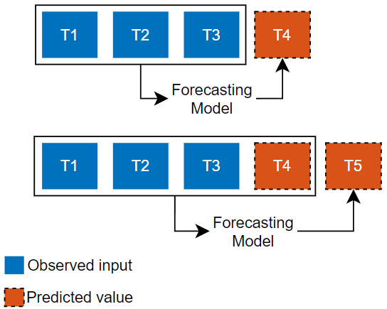
Predict the next time step in a sequence using only the input data. When making predictions for subsequent time steps, you collect the true values from your data source and use those as input. Use this type of prediction when you have true values to provide to the model before making the next prediction. For example, use this option if you want to predict the next day's temperature, where each day you can record the true temperature value and use it as input to your model.	Predict subsequent time steps in a sequence by using the previous predictions as input. In this case, the model does not require the true values to make the prediction. Use this type of prediction to predict multiple subsequent time steps or when you do not have the true values to provide to the RNN before making the next prediction. For example, use this option if you have a virtual sensor and do not have access to live values to use as input to your model at each time step.

Dependencies

This option appears only for ARMAX models, nonlinear ARX models, and when you select Use past values of responses as inputs (use an autoregressive model) for deep learning models.

Data source — Data to predict values for

Validation (default) | Training

Use the Data source list to select which data to predict with. The performance of the model on the validation data is usually a more accurate reflection of how the model will perform on new data than the performance of the model on the training data.

Use stateful prediction — Flag to use stateful prediction

'off' | 'on'

This option is only available for deep learning models.

Select the Use stateful prediction check box to update the network state every iteration during closed loop prediction. Select this option if your model architecture supports statefulness (for example, LSTM or GRU) and you want to maintain the state of the network between iterations.

Dependencies

This options is available only if Prediction type is set to Closed loop and only for the Predict, Residuals, and Residual Histogram plots.

The default Use stateful prediction value depends on the network and the Sliding window length value. For most networks, using stateful prediction with a sliding window length value greater than 1 will produce poor results. By default, the app does not use stateful prediction if the sliding window length is greater than one.

Sliding window length — Length of sliding window

'off' | 'on'

This option is only available for deep learning models.

Specify the number of time steps to use as input at each subsequent prediction step during closed loop prediction. After the initial prediction, the model slides through the time series as it makes predictions. Choose a window length that captures enough information to make the prediction. A window length that is too short can cause the model to miss trends, and a window length that is too long can add noise or complexity to the predictions. If you have only output data, then you might need a longer window length in order to make accurate predictions.

Dependencies

This option is available only if Prediction type is set to Closed loop and only for the Predict, Residuals, and Residual Histogram plots.

Overlay normal distribution — Overlay the normal distribution on the residuals histogram

checkbox

Overlay a normal distribution with mean 0 and standard deviation of σ, where σ is the standard deviation of the residuals.

Dependencies

This option is available only for the Residual Histogram plot.

Export — Export trained network

button

Click the Export button to export the trained model and the training statistics to the MATLAB workspace and generate a live script for predicting on new data. For deep learning models, the app exports a structure array that contains the model as a dlnetwork (Deep Learning Toolbox) object. For the ARMAX model, the app exports a structure that contains an idpoly model. For the nonlinear ARX model, the app exports a structure that contains an idnlarx model. The generated live script contains code for preparing and normalizing data and predicting values for new data.

Export to Workspace and Generate Code — Export trained model and generate script for prediction

button

This button has the same effect as the Export button.

Export to Workspace — Export trained model

button

Click the Export to Workspace button to export the trained model to the MATLAB workspace. For deep learning models, the app exports the network as a dlnetwork (Deep Learning Toolbox) object. For the ARMAX model, the app exports a structure that contains an idpoly model. For the nonlinear ARX model, the app exports a structure that contains an idnlarx model.

Export to Simulink — Export trained model to Simulink

button

Click the Export to Simulink button to export the trained model to Simulink. For deep learning models, the app exports the model as layer blocks. The app reports if any layers are not supported as layer blocks. For more information, see List of Deep Learning Layer Blocks and Subsystems (Deep Learning Toolbox).

In the dialog box, you can specify the sample time for the generated model. To specify the sample time, select Specify a fixed-step size and enter the step size as a positive scalar. The sample time controls how the model operates in simulations. For more information about sample time in Simulink, see Specify Sample Time (Simulink).

For the ARMAX model, the app exports the model as an Idmodel block. For the nonlinear ARX model, the app exports the model as a Nonlinear ARX Model block. For more information, see Export Trained Model.

Version History

Introduced in R2026b